Robust Model Reference Adaptive Control

Motivation

In the design of vehicle control system, it is essential to provide closed-loop stability, adequate command tracking performance, as well as robustness to model uncertainties, control failures and environmental disturbances. However, in the presence of matched uncertainties, a deterioration of the system nominal(baseline) control is inevitable. We pose the question:”Can we restore a given nominal closed-loop performance of the system, while operating under matched uncertainties?”

Problem Setup

Without loss of generality, we define open loop system dynamics in the form of

\[\dot{x}_p=A_px_p+B_p\Lambda u +B_p\delta_p(x_p)\]

where $A_p,B_p$ are known system matrix, $x_p$ is system states, $u$ is control.

Dimensionality:

\[\begin{aligned} x_p &\in \Re^{n_p \times 1} \\ A_p &\in \Re^{n_p \times n_p} \\ B_p &\in \Re^{n_p \times m} \\ \Lambda &\in \Re^{m \times m} \\ u &\in \Re^{m \times1} \\ \delta_p &\in \Re^{m \times 1} \\ \end{aligned}\]

$\Lambda$ is unknown control effectiveness uncertainty and is defined as

\[\Lambda = \left[ \begin{matrix} \Lambda_1 & 0 & \cdots & 0 \\ 0 & \Lambda_2 & \cdots & 0 \\ \vdots & \vdots & \ddots & \vdots \\ 0 & 0 & \cdots & \Lambda_m \\ \end{matrix} \right] \succ0\]

$\delta_p(x_p)$ is non-linear system uncertainty and is defined as

\[\begin{aligned} &\delta_p(x_p)=W_p^T \sigma_p(x_p)\\& \end{aligned}\]

Dimensionality:

\[\begin{aligned} \delta_p &\in \Re^{m \times 1}\\ W_p &\in \Re^{n_s \times m}\\ \sigma_p &\in \Re^{n_s \times 1} \end{aligned}\]

where $W_p$ is unknown weights, $\sigma_p$ is known basis function which is defined as

\[\begin{aligned} &\sigma_p(x_p)=[\sigma_{p_1}(x_p) \ \cdots \ \sigma_{p_s}(x_p)] \\ &\sigma_{p_i}: \Re^{n_p\times1} \to \Re^{n_s\times1},\text{ a locally lipschitz function} \end{aligned}\]

Thus we can rewrite system dynamics as

\[\dot{x}_p=A_px_p+Bp\Lambda[u + \Lambda^{-1}B_p\delta_p(x_p)]\]

which indicates control $u$ can access all uncertainties.

Assume

\[u = u_n + u_a\]

where $u_n$ is nominal control which is designed for perfectly modeled system without uncertainty and $u_a$ is adaptive control which is designed to handle all system uncertainties.

Now, let’s design nominal control for ideal system.

\[u = u_n + u_a = u_n = -K_xx_p+K_rr\]

where $K_x$ is feedback gain, $ x_p$ is feedback state, $ K_r$ is feedforward gain, $ r$ is feedforward command.

Dimensionality

\[\begin{aligned} x_p &\in \Re^{n_p \times 1} \\ K_x &\in \Re^{m \times n_p} \\ r &\in \Re^{n_c \times 1} \\ K_r &\in \Re^{m \times n_c} \\ \end{aligned}\]

plug into ideal system,we have

\[\begin{aligned} \dot{x}_p&=A_px_p+B_pu_n\\ &=A_px_p+B_p(-K_xx_p+K_rr)\\ &=(A_p-B_pK_x)x_p+B_pK_rr\\ &=A_rx_p+B_rr \end{aligned}\]

Therefore, we define Reference Model as

\[\dot{x}_r = A_rx_r+B_rr\]

Now, let’s consider model selection with uncertainty

\[\begin{aligned} \dot{x}_p &=A_px_p+B_p\Lambda u +B_p\delta_p(x_p)\\ &=A_px_p+B_p\Lambda[u_n+u_a]+B_p\delta_p(x_p)\\ &=A_px_p+B_p\Lambda[u_n+u_a]+B_p\delta_p(x_p)+\color{red}{B_pK_xx_p-B_pK_xx_p+B_pK_rr-B_pK_rr}\\ &=(A_p-B_pK_x)x_p+B_pK_rr+B_p\Lambda[u_n+u_a+\Lambda^{-1}W_p^T\sigma_p(x_p)-\Lambda^{-1}(-K_xx_p+K_rr)]\\ &=A_rx_p+B_rr+B_p\Lambda[u_n+u_a+\Lambda^{-1}W_p^T\sigma_p(x_p)-\Lambda^{-1}u_n]\\ &=A_rx_p+B_rr+B_p\Lambda[(I-\Lambda^{-1})u_n+\Lambda^{-1}W_p^T\sigma_p(x_p)+u_a] \end{aligned}\]

define

\[\begin{aligned} &W\triangleq[\Lambda^{-1}W_p^T\quad I-\Lambda^{-1}]^T\\ &\sigma(x_p,u_n)\triangleq[\sigma_p(x_p)\quad u_n]^T \end{aligned}\]

formally, we get

\[\dot{x}_p=\color{green}{A_rx_p+B_rr}+\color{red}{B_p\Lambda[W^T\sigma(x_p,u_n)+u_a]}\]

where green part represents desire(reference) dynamics, red part represents adaptive term

Apparently we want to make red term equals to zero, thus

\[u_a=-\hat{W}^T\sigma\]

where $\hat{W}$ is the estimation of ground truth weight $W$

define

\[\begin{aligned} &\widetilde{W}=\hat{W}-W\\ &u_a+W^T\sigma=-\hat{W}^T\sigma(x_p,u_n)+W^T\sigma=-\widetilde{W}\sigma \end{aligned}\]

finally we get

\[\dot{x}_p=\color{green}{A_rx_p+B_rr}-\color{red}{B_p\Lambda\widetilde{W}^T\sigma}\]

Error Dynamics

define

\[e \triangleq x_p - x_r\]

therefore, the error dynamics is

\[\begin{aligned}\dot{e} &=\dot{x}_p-\dot{x}_r\\ &=A_rx_p+B_rr-B_p\Lambda\widetilde{W}^T\sigma-A_rx_r-B_rr\\ &=A_re-B_p\Lambda\widetilde{W}^T\sigma \end{aligned}\]

Adaption Law based on Lyapunov Theorem

Lyapunov Second Method states:

Consider a function $V(x) : \Re_n \to \Re$ such that

\[\begin{aligned} &V(x) \succeq 0 ,\quad = \text{ only holds at equilibrium}\\ &\dot{V}(x(t)) \prec 0 \end{aligned}\]

Then we conclude that $V(x)$ is called Lyapunov candidate and the system is stable in sense of Lyapunov(ISL).

The next step is select parameter adjustment mechanism for $\widetilde{W}$ , such that

\[\lim_{t \to \infty}e = 0\]

We start with Lyapunov function, the Lyapunov candidate we choose for adaptive control is

\[V=e^TPe+\gamma^{-1}tr(\widetilde{W}\Lambda^{\frac{1}{2}})^Ttr(\widetilde{W}\Lambda^{\frac{1}{2}})\]

where $\gamma$ is a positive real number which represents learning rate, and $P$ is a positive definite matrix ($P \succ 0)$ which satisfy following continuous Lyapunov Equation:

\[A_r^TP+PA_r=-Q\]

where $Q$ is positive definite ($Q \succ 0$) and $A$ is Hurwitz ($Re(\lambda) \prec 0$)

From the equation above, we can conclude that $V \succ 0$.

Before moving on, let’s take some useful mathematic sidenotes

where $Q$ is positive definite ($Q \succ 0$) and $A$ is Hurwitz ($Re(\lambda) \prec 0$)

From the equation above, we can conclude that $V \succ 0$.

Before moving on, let’s take some useful mathematic sidenotes

\[\begin{aligned} &tr(ab)=tr(ba)=ab\\ &tr(a+b)=tr(a)+tr(b) \end{aligned}\]

Now let’s analysis $\dot{V}$

\[\begin{aligned} \dot{V} &=e^TP\dot{e}+\dot{e}^TPe+2\gamma^{-1}tr(\Lambda\widetilde{W}^T\dot{\hat{W}})\\ &=e^TP(A_re-B_p\Lambda\widetilde{W}^T\sigma)+(A_re-B_p\Lambda\widetilde{W}^T\sigma)^TPe+2\gamma^{-1}tr(\Lambda\widetilde{W}^T\dot{\hat{W}})\\ &=e^T(PA_r+A_r^TP)e-2e^TPB_p\Lambda\widetilde{W}^T\sigma+2\gamma^{-1}tr(\Lambda\widetilde{W}^T\dot{\hat{W}})\\ &=-e^TQe-2tr(\Lambda\widetilde{W}^T\sigma e^TPB_p)+2\gamma^{-1}tr(\Lambda\widetilde{W}^T\dot{\hat{W}})\\ &=-e^TQe-2\gamma^{-1}tr(\gamma\Lambda\widetilde{W}^T\sigma e^TPB_p-\Lambda\widetilde{W}^T\dot{\hat{W}})\\ &=-e^TQe-2\gamma^{-1}tr(\Lambda\widetilde{W}^T(\gamma\sigma e^TPB_p-\dot{\hat{W}})) \end{aligned}\]

we already know that $Q\succ0$,thus we select adaption law as

\[\color{red}{\dot{\hat{W}}=\gamma\sigma e^TPB_p}\]

In such case, we have

\[\dot{V}=-e^TQe\prec0\]

Also we observe that adaption law is nothing but learning rate $\times$ states $\times e^TpB_p$ and model reference adaptive control is nothing but non-linear integral control.

According to Lyapunov $2^nd$ Theorem, we can conclude that

\[(e,\widetilde{W}) \in L_{\infty}(\text{bounded and stable})\]

Furthermore, we can analysis second derivative of $V$ ,

\[\begin{aligned} \ddot{V} &=-[e^TQ\dot{e}+\dot{e}^TQe] \\ &=-[e^TQ(A_re-B_p\Lambda\widetilde{W}^T\sigma(e+x_r,u_n))+(A_re-B_p\Lambda\widetilde{W}^T\sigma(e+x_r,u_n))^TQe] \end{aligned}\]

Since $e,x_r,u_n$ are bounded, $A_r$ is Hurwitz, $\widetilde{W} = \hat{W} - W = \hat{W} - Constant$ is bounded. According to Barbalet Lemma, we can conclude that

\[\begin{aligned} &\because\ddot{V} \text{ is bounded} \\ &\therefore\dot{V} = -e^TQe \to 0 \quad\text{as}\quad t \to \infty \quad(\lim_{t \to \infty}e(t)=0)\\ &\text{which is known as UUB(uniformly ultimately boundness) condition } \quad\to\quad \\ &\text{system state tracks the state of reference model globally and asymptotically} \\ & \end{aligned}\]

It’s important to notice that $\widetilde{W} \to 0$ as $t \to \infty$ ,is not guaranteed, which means the adaptive parameters are not guaranteed to converge to their true unknown values, nor they are assured to converge to constant values in any way.(Actually, it should satisfy certain conditions(Persistent Excitation) to achieve that, we will not discuss here). To conclude, it is not ideal for parameter estimation(system identification).

Summarize

Standard MRAC

\[\begin{aligned} \text{System Dynamics}& \\ &\dot{x}_p=A_px_p+B_p\Lambda u +B_p\delta_p(x_p)\\ \text{Total Control Law}& \\ &u = u_n + u_a \\ \text{Nominal Control Law}\\ &u_n = -K_xx_p + K_rr \\ &A_r = A_p - B_pK_x \\ &B_r = B_pK_r \\ \text{Adaptive Control Law} \\ &u_a=-\hat{W}^T\sigma\\ &\dot{\hat{W}}=\gamma\sigma e^TPB_p=\gamma\sigma (x_p-x_r)^TPB_p\\ &\sigma(x_p,u_n)\triangleq[\sigma_p(x_p)\quad u_n]^T\\ &\dot{x}_r=A_rx_r+B_rr\\ &A_r^TP+PA_r=-Q\\ \end{aligned}\]

Improve Transient Dynamics

Recall error dynamics:

\[\begin{aligned}\dot{e} &=\dot{x}_p-\dot{x}_r\\ &=A_rx_p+B_rr-B_p\Lambda\widetilde{W}^T\sigma-A_rx_r-B_rr\\ &=A_re-B_p\Lambda\widetilde{W}^T\sigma \end{aligned}\]

Note that reference dynamics and error dynamics share same system matrix $A_r$. This might cause oscillation when learning rate is big. To address this problem,we need to make error dynamics faster than reference model. We can achieve arbitrarily fast error dynamics by adding an error feedback term into reference model just like designing a state observer. The modified reference model is as follow:

\[\dot{x}_r = A_rx_r+B_rr+L_v(x_p-x_r) = A_rx_r+B_rr+L_ve\]

where $L_v$ is a positive observer gain.

Then, the corresponding error dynamics is:

\[\begin{aligned}\dot{e} &=\dot{x}_p-\dot{x}_r\\ &=A_rx_p+B_rr-B_p\Lambda\widetilde{W}^T\sigma-A_rx_r-B_rr-L_ve\\ &=(A_r-L_v)e-B_p\Lambda\widetilde{W}^T\sigma \end{aligned}\]

define $A_v = A_r-L_v$

\[\dot{e}=A_ve-B_p\Lambda\widetilde{W}^T\sigma\]

Theoretically, we can make error dynamics arbitrarily fast by subtracting a positive infinite $L_v$ gain from reference system matrix $A_r$. However the analytical stability properties of closed-loop system must be preserved. So the next question is: What is the proper parameter adjusting mechanism of $L_v$ gain for the error dynamics? Well, it seems a good idea to borrow it from observer design.

We choose $L_v = P_vR_v^{-1}$ where $P_v = P_v^T \succ0$ is the unique solution of the filter algebraic Riccati equation with identity $C_v$ matrix.

The FARE(filter algebraic Riccati equation) is written as follow:

\[\begin{aligned} &P_vA_r^T+A_rP_v - P_vC_v^TR_v^{-1}C_vP_v + Q_v = 0, \quad C_v = I_{nxn} \text{ in our cases}\\ &P_vA_r^T+A_rP_v - P_vR_v^{-1}P_v + Q_v = 0 \end{aligned}\]

with the ARE weight matrices $(Q_v,R_v)$ select as

\[\begin{aligned} Q_v &= Q_0 + \frac{v+1}{v}I_{nxn} \\ R_v &= \frac{v}{v+1}I_{nxn} \\ L_v &= P_vR_v^{-1}=(1+\frac{1}{v})P_v \end{aligned}\]

where $v$ is a positive real scalar. Therefore, $L_v \to \infty \text{ as } v \to 0$, which leads to faster error dynamics.

Now, we substitute $L_v$ with $P_vR_v^{-1}$ and rewrite filter algebraic Riccati equation in terms of $A_v$, we can get following results:

\[\begin{aligned} &P_v(A_r-P_vR_v^{-1})^T+(A_r-P_vR_v^{-1})P_v + P_vR_v^{-1}P_v + Q_v = 0\\ &P_vA_v^T + A_vP_v = -Q_v - P_vR_v^{-1}P_v \prec 0 \end{aligned}\]

Now, let’s analysis the stability properties of this adaptive system. The Lyapunov candidate we select is:

\[V=e^TPe+\gamma^{-1}tr(\widetilde{W}\Lambda^{\frac{1}{2}})^Ttr(\widetilde{W}\Lambda^{\frac{1}{2}})\]

And its derivative is:

\[\begin{aligned} \dot{V} &=e^TP\dot{e}+\dot{e}^TPe+2\gamma^{-1}tr(\Lambda\widetilde{W}^T\dot{\hat{W}})\\ &=e^TP(A_ve-B_p\Lambda\widetilde{W}^T\sigma)+(A_ve-B_p\Lambda\widetilde{W}^T\sigma)^TPe+2\gamma^{-1}tr(\Lambda\widetilde{W}^T\dot{\hat{W}})\\ &=e^T(PA_v+A_v^TP)e-2e^TPB_p\Lambda\widetilde{W}^T\sigma+2\gamma^{-1}tr(\Lambda\widetilde{W}^T\dot{\hat{W}})\\ &=e^T(PA_v+A_v^TP)e-2tr(\Lambda\widetilde{W}^T\sigma e^TPB_p)+2\gamma^{-1}tr(\Lambda\widetilde{W}^T\dot{\hat{W}})\\ &=e^T(PA_v+A_v^TP)e-2\gamma^{-1}tr(\gamma\Lambda\widetilde{W}^T\sigma e^TPB_p-\Lambda\widetilde{W}^T\dot{\hat{W}})\\ &=e^T(PA_v+A_v^TP)e-2\gamma^{-1}tr(\Lambda\widetilde{W}^T(\gamma\sigma e^TPB_p-\dot{\hat{W}})) \end{aligned}\]

As we discussed before, we select adaptive law as

\[\dot{\hat{W}}=\gamma\sigma e^TPB_p\]

Then

\[\dot{V} = e^T(PA_v+A_v^TP)e = -Q_v - P_vR_v^{-1}P_v \prec 0\]

Hence the system is stable ISL.

Attack to Steering/Throttle/Brake Problem with MRAC

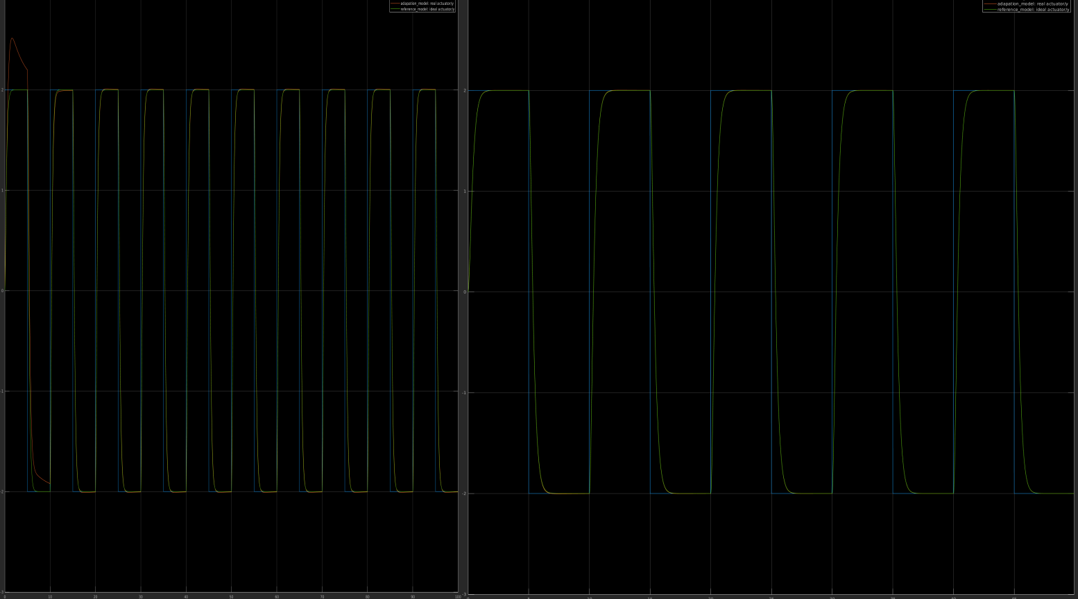
In previous section,we design MRAC adaption law by Lyapunov Stability Theorem in most common case and found its error dynamics satisfies UUB condition and all states are uniformly bounded in time. Now let’s design a model reference adaptive controller for vehicle longitudinal and lateral control.Let’s take longitudinal MRAC as example,the motivation of this project is to achieve better inner loop performance(acceleration tracking performance) in the presence of various system uncertainties (non-linear actuator,inaccurate calibration table,non-ideal road conditions). Our goal is design a controller which will learn the system uncertainties and recover ideal performance from it.

In this project,we identificate throttle and brake dynamics as second-order system (plant model) as follow

\[\begin{aligned} &\dot{x}_p = A_px_p+B_pu\\ \\ &\left[ \begin{matrix} \dot{x}_{p_1}\\ \dot{x}_{p_2}\\ \end{matrix} \right] = \left[ \begin{matrix} 0 & 1\\ -w_p^2 &-2\eta_p w_p \end{matrix} \right] \left[ \begin{matrix} x_{p_1}\\ x_{p_2} \end{matrix} \right] + \left[ \begin{matrix} 0\\ w_p^2 \end{matrix} \right]u \end{aligned}\]

Though real throttle and brake dynamics might not be a second-order system,we could encode its main properties (rising time,dead time,damping,etc) by a simple second-order system. It doesn’t matter how accurate it is cause the goal is to track reference model,in this case,a ideal throttle and brake dynamics.

The reference model is also a second-order system modeled as following

\[\begin{aligned} &\dot{x}_r = A_rx_r+B_rr\\ \\ &\left[ \begin{matrix} \dot{x}_{r_1}\\ \dot{x}_{r_2}\\ \end{matrix} \right] = \left[ \begin{matrix} 0 & 1\\ -w_r^2 &-2\eta_r w_r \end{matrix} \right] \left[ \begin{matrix} x_{r_1}\\ x_{r_2} \end{matrix} \right] + \left[ \begin{matrix} 0\\ w_r^2 \end{matrix} \right]r \end{aligned}\]

There is no big difference here,we use different subscript to represents different values.

Now,we need to design control law $u$ to make real system behave just like reference model,we select

\(u=W_x^Tx_p+W_r^Tr\) Assume there exist ideal gain $W_x^*$ and $W_r^*$ such we can perfectly tracking the reference model,thus \(\begin{aligned} &A_rx_r+B_rr = A_px_p+B_pu^* ,(x_p = x_r)\\ &(A_r-A_p)x_r+B_rr-B_p(W_x^{*^T}x_r+W_r^{*^T}r)=0\\ &[(A_r-A_p)-B_pW_x^{*^T}]x_r+(B_r-B_pW_r^{*^T})r=0\\ \\ &W_x^{*^T} = B_p^{\dagger}(Ar-A_p)\\ &W_r^{*^T} = B_p^{\dagger}B_r \\ \\ &A_r = A_p + B_pW_x^{*^T}\\ &B_r = B_pW_r^{*^T} \end{aligned}\)

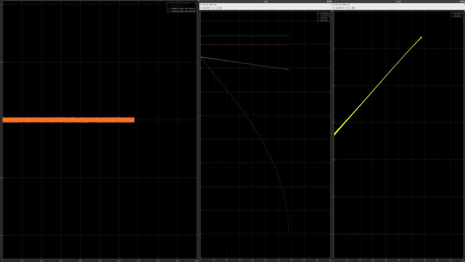
From above,we know that if we have some pre-known knowledge about plant dynamics,we can estimate the ideal gain $W_x^*$ and $W_r^*$ and set it as initial condition. Initial condition is very important influence factors on performance of the MRAC,let’s take a look

Alright,let’s continue. $A_p$ and $B_p$ are unknown here(in the contrast to previous section),we need to estimate them,so the control we have is

\[u=\hat{W}_x^Tx_p+\hat{W}_r^Tr\]

define

\[\begin{aligned} \widetilde{W}_x &= \hat{W}_x - W_x^*\\ \widetilde{W}_r &= \hat{W}_r - W_r^* \end{aligned}\]

Plug into plant model,we have

\[\begin{aligned} \dot{x}_p&=A_px_p+B_p(\hat{W}_x^Tx_p+\hat{W}_r^Tx_r)\\ &=A_px_p+B_p(\hat{W}_x^Tx_p+\hat{W}_r^Tx_r+\color{red}{W_x^{*^T}x_p-W_x^{*^T}x_p+W_r^{*^T}r-W_r^{*^T}r})\\ &=A_px_p+B_pW_x^{*^T}x_p+B_pW_r^{*^T}r+B_p[(\hat{W}_x - W_x^*)^Tx_p+(\hat{W}_r - W_r^*)^Tr]\\ &=\color{green}{A_rx_p+B_rr}+\color{red}{B_p(\widetilde{W_x}^Tx_p+\widetilde{W}_r^Tr)} \end{aligned}\]

Now let’s consider error dynamics

define

\[e \triangleq x_p-x_r\]

then we have

\[\begin{aligned} \dot{e} &=\dot{x}_p-\dot{x}_r\\ &=A_rx_p+B_rr+B_p(-\widetilde{W_x}^Tx_p+\widetilde{W}_r^Tr) - A_rx_r - B_rr\\ &=A_re+B_p(\widetilde{W_x}^Tx_p+\widetilde{W}_r^Tr) \end{aligned}\]

Next we design parameter adjustment mechanism for $\widetilde{W}_x$ and $\widetilde{W}_r$ based on Lyapunov Stability Theorem,choose Lyapunov function as

\[V=e^TPe+\gamma_x^{-1}\widetilde{W_x}^T\widetilde{W_x}+\gamma_r^{-1}\widetilde{W_r}^T\widetilde{W_r}\]

where $\gamma_x$ is learning rate for state feedback, $\gamma_r$ is learning rate for input feedforward,,and $P$ is a positive definite matrix $(P\succ0)$ which satisfy following continuous Lyapunov Equation:

\[A_r^TP+PA_r=-Q\]

where $Q$ is positive definite $(Q\succ0)$

Now let’s analysis $\dot{V}$,skip the math we can get

\[\dot{V} = -e^TQe+2\widetilde{W_x}^T(x_pe^TPB_p+\gamma_x^{-1}\dot{\widetilde{W}_x})+2\widetilde{W_r}^T(re^TPB_p+\gamma_r^{-1}\dot{\widetilde{W}_r})\]

thus we select adptive law as

\[\begin{aligned} \dot{\widetilde{W}_x} &= -\gamma_xx_pe^TPB_p\\ \dot{\widetilde{W}_r} &= -\gamma_rre^TPB_p \end{aligned}\]

so that

\[\dot{V}\prec0\]

Parameter Drifting: The Sudden Failure

Plant model with uniformly bounded disturbances

\[\dot{x}_p=A_px_p+B_pu+\xi(t),\quad\xi(t)\le\xi_{max}\]

Reference model

\[\dot{x}_r=A_rx_r+B_rr\]

Adaptive law

\[u=\theta_x^Tx_p+\theta_r^Tr\]

Rewrite plant mode

\[\begin{aligned} &A_px+B_p(\theta_x^{\ast T}x + \theta_r^{\ast T}r)=A_rx+B_rr \\ \\ &\left\{ \begin{aligned} A_p+B_p\theta_x^{\ast T}&=Ar \\ B_p\theta_r^{\ast T}&=Br \end{aligned} \right.\\ \\ & \begin{aligned} \dot{x}_p &=A_px_p+B_p(\theta_x^Tx_p+\theta_r^Tr+\theta_x^{\ast T}x_p-\theta_x^{\ast T}x_p+\theta_r^{\ast T}r-\theta_r^{\ast T}r)+\xi(t) \\ &=(A_p+B_p\theta_x^{\ast T})x_p+B_p\theta_r^{\ast T}r+B_p(\theta_x^T-\theta_x^{\ast T} + \theta_r^T-\theta_r^{\ast T})+\xi(t) \\ &=A_rx_p+B_rr+B_p(\Delta\theta_x^Tx_p+\Delta\theta_r^Tr)+\xi(t) \end{aligned} \end{aligned}\]

Error dynamics

\[\begin{aligned} &e\triangleq x_p-x_r\\ &\dot{e}=A_re+B_p(\Delta\theta_x^Tx_p+\Delta\theta_r^Tr)+\xi(t)\\ \\ &let\quad \theta= \begin{bmatrix} \theta_r \\ \theta_x \end{bmatrix}\quad \Gamma_\theta= \begin{bmatrix} \Gamma_x & 0 \\ 0 & \Gamma_r \end{bmatrix}\quad \Delta\theta= \begin{bmatrix} \Delta\theta_r \\ \Delta\theta_x\end{bmatrix}\quad \phi= \begin{bmatrix} r \\ x \end{bmatrix}\\ \\ &\dot{e} = A_re+B_p\Delta\theta^T\phi+\xi(t) \end{aligned}\]

Analysis Lyapunov stability

\[\begin{aligned} &V=e^TPe+tr(\Delta\theta^T\Gamma_\theta^{-1}\Delta\theta)\\ \\ & \begin{aligned} \dot{V}&=\dot{e}^TPe+e^tP\dot{e}+2tr(\Delta\theta^T\Gamma_\theta^{-1}\dot\theta)\\ &=(A_re+B_p\Delta\theta^T\phi+\xi)Pe+e^TP(A_re+B_p\Delta\theta^T\phi+\xi)+2tr(\Delta\theta^T\Gamma_\theta^{-1}\dot\theta)\\ &=e^T(A_r^TP+PA_r)e+2e^TPB_p\Delta\theta^T\phi+2tr(\Delta\theta^T\Gamma_\theta^{-1}\dot\theta)+\color{red}{2e^TP\xi} \\ &=-e^TQe+2tr(\Delta\theta^T(\Gamma_\theta^{-1}\dot\theta+\phi e^TpB_p))+\color{red}{2e^TP\xi} \end{aligned} \end{aligned}\]

Base on equation above,we choose MRAC adaption law as

\[\dot{\theta}=-\Gamma_\theta\phi e^TPB_p\]

thus we have

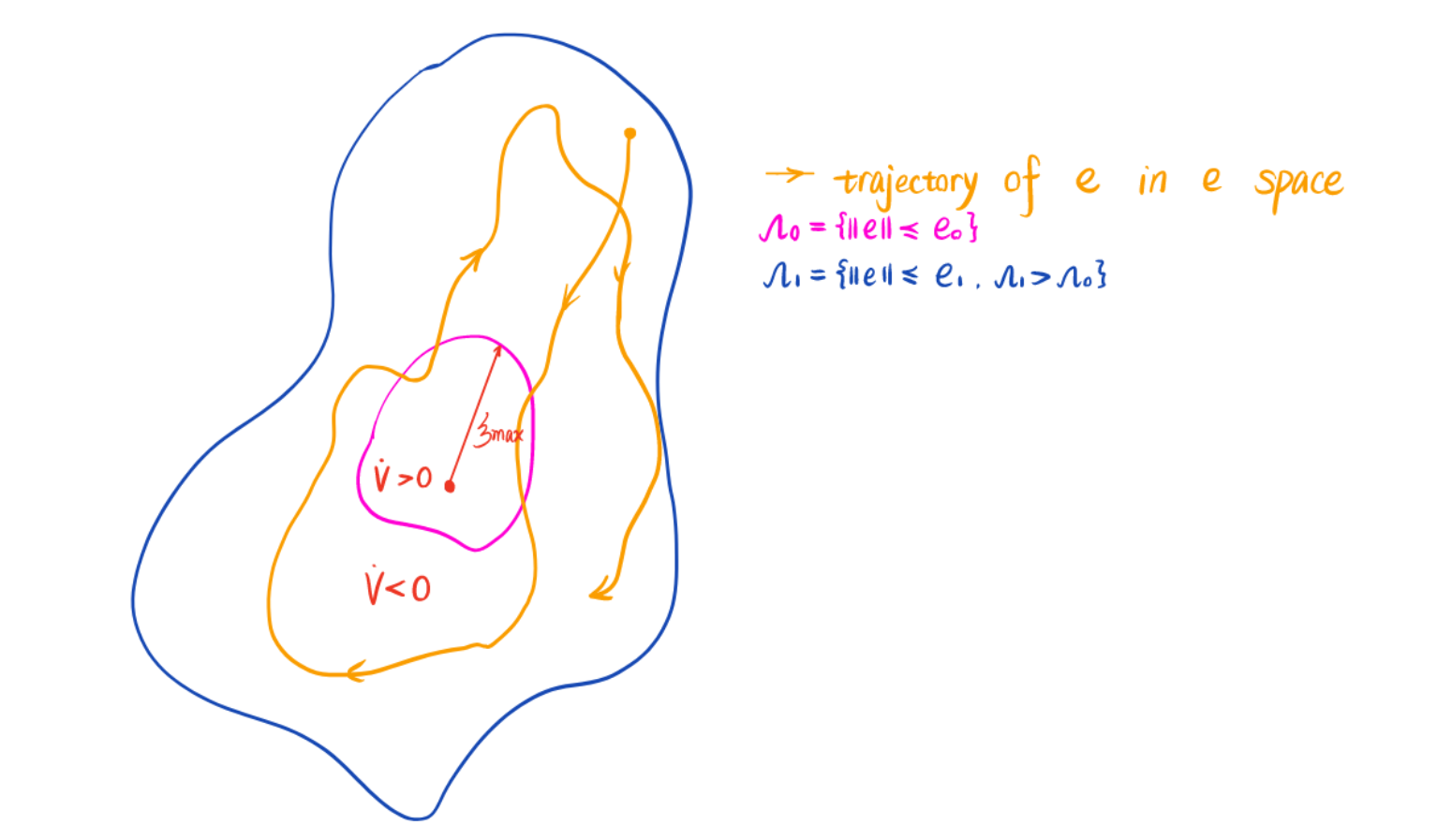
\[\begin{aligned} &\dot{V}=-e^TQe+2e^TP\xi \le -\lambda_{min}(Q)\Vert e \Vert_{l_2}^2+2\Vert e \Vert_{l_2}\lambda_{max}(P)\xi_{max} \\ \\ &\dot V < 0 \quad \text{is always true outside of set} \ \Omega_0 \\ \\ &\Omega_0:\{\Vert e\Vert_{l_2} \le \frac{2\lambda_{max}(P)\xi_{max}}{\lambda_{min}(Q)}:= e_0 \} \end{aligned}\]

If state tracking error enters compact set $\Omega_1$ in finite time,it will remain inside for all future time. Note that $\Omega_0$ is compact in e space,however not compact in $\Delta\theta$ space. Therefore $\Delta\theta$ is not restricted at all. Inside $\Omega_0$, $\dot{V}$ can be positive,as a consequence, $\Delta\theta$ can grow unbounded even though e is bounded. This is known as “Parameter Drifting”.This shows that MRAC law $\dot{\theta}=-\Gamma_\theta\phi e^TPB_p$ is not robust to bounded disturbances,no matter how small the latter are.

In order to resolve this problem,we need to pose a constraint for $\Delta\theta$ to make it stays in a compact set. But how? There are several methods to attack this problem.

deadzone-Modification

First method is simple and effective,note that drifts are caused by bounded disturbances in our case,so stop adaption when error is small enough might be a good strategy,so the modified adaption law is

\[\begin{aligned} &\dot{\hat\theta}=\Gamma_\theta(\phi(x)\mu(\Vert e\Vert) e^TPB_p)\\ \\ &\mu(\Vert e\Vert) = \left\{ \begin{aligned} 1,\quad \Vert e \Vert > \xi_{max}\\ 0,\quad \Vert e \Vert \leq \xi_{max} \end{aligned} \right.\\ \end{aligned}\]

Well,it does help but the price is that we get bounded tracking.

e-Modification

Furthermore,we can prevent high-frequency adaption by adding damping,the modified adaption law becomes

\[\dot{\hat\theta}=\Gamma_\theta(\phi(x)e^TPB_p-\sigma\hat\theta)\]

Take the Laplace Transform of previous adaption law,we have

\[\begin{aligned} s{\hat\theta} + \Gamma_\theta\sigma\hat\theta &=\Gamma_\theta\phi(x)e^TPB_p \\ \hat\theta &=\frac{1}{s+\Gamma_\theta\sigma}\Gamma_\theta\phi(x)e^TPB_p\\ &=\text{Lowpass Filter} * \Gamma_\theta\phi(x)e^TPB_p \end{aligned}\]

However it is not good enough,because it slows down the adaption. In order to achieve fast adaption when error is relatively small,we improve previous adaption law by adding a e term into damping,the e-Modification adaption law is

\[\dot{\hat\theta}=\Gamma_\theta(\phi(x)e^TPB_p-\sigma\Vert e^TPB_p \Vert\hat\theta)\]

Projection Modification

However,we still cannot handle nonparametric uncertainties because there is no constraint for $\Delta\theta$. In order to achieve fast adaption,enforce uniformly boundness of adaptive parameters and maintain closed-loop stability of error dynamics and original system,introducing prjection modification of adaption law. The projection-modification adaption law is

\[\begin{aligned} &\dot{\hat\theta} = proj(\hat\theta,-\Gamma_\theta\phi e^TPB_p)\\ \\ &\text{in our second-order system case,the adaption law is }\\ &\dot{\hat\theta}_x = proj(\hat\theta_x,-\Gamma_xxe^TPB_p)\\ &\dot{\hat\theta}_r = proj(\hat\theta_r,-\Gamma_rre^TPB_p) \end{aligned}\]

Projection Operator

The projection operator is represented by equation:

\[\begin{equation} proj(\theta,\Gamma y) = \left\{\begin{aligned}\frac {\Gamma\nabla{f}(\nabla{f})^T}{(\nabla{f})^T\Gamma\nabla{f}} yf & & {f>0\land y^T\nabla{f}>0}\\ y & & {otherwise}\end{aligned}\right.\end{equation}\]

where $f(\theta)$ is a convex boundary function,we choose $f(\theta)$ as follow

\[f(\theta)=\frac{(1+\varepsilon)\theta^T\theta - \Vert\theta\Vert^{max}}{\varepsilon\Vert\theta\Vert^{max}}\]

What does projection operator do?

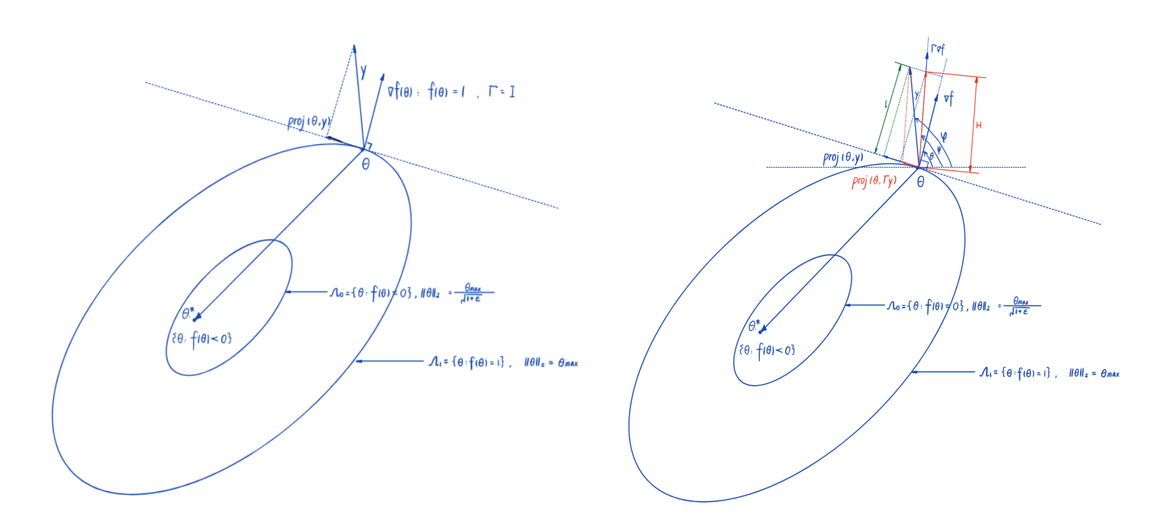
Here,we assume that the ground turth $\theta^*$ lives in a compact set ,so make sure $\theta^*$ is inside of preselected convex set $\Omega_1$

Convex Property of Projection Operator

\[(\theta-\theta^*)^T(\Gamma^{-1}proj(\theta,\Gamma y)-y)\le 0\]

thus

\[\begin{aligned} &tr(\Delta\theta^T(\Gamma^{-1}proj(\hat\theta,\Gamma Y)-Y))=\sum_{j=1}^m(\hat\theta-\theta)_j^T(\Gamma^{-1}proj(\hat\theta,\Gamma Y_j)-Y_j)\le 0 \\ \\ & \begin{aligned} tr(\Delta\theta^T(\Gamma_\theta^{-1}\dot{\hat\theta}-\phi e^TpB_p)) &=tr((\theta - \theta^*)(\Gamma_\theta^{-1}proj(\hat\theta,\Gamma_\theta\phi e^TPB_p)-\phi e^TPB_p)) \\ &= \sum_{j=1}^m(\hat\theta-\theta^*)_j^T(\Gamma^{-1}proj(\hat\theta,\Gamma Y_j)-Y_j)\le 0 \end{aligned} \end{aligned}\]

Combining with Lyapunov function we derived above,we have

\[\begin{aligned} \dot{V} &=-e^TQe+2tr(\Delta\theta^T(\Gamma_\theta^{-1}\dot\theta-\phi e^TpB_p))+2e^TP\xi \\ &\le-e^TQe+2e^TP\xi \\ &\le-\lambda_{min}(Q)\Vert e \Vert_{l_2}^2+2\Vert e \Vert_{l_2}\lambda_{max}(P)\xi_{max} \end{aligned}\]

Comparing to the $\dot{V}$ we derived from Parameter Drifting section,we can conclude that projection operator maintain the stability of error dynamics and original system.

Summarize

The prjection-based MRAC adaption law has following properties:

\[\begin{aligned} &\text{1.Fast adaption}\\ &\text{2.Enforce uniformly boundness of adaptive parameters}\\ &\text{3.Maintain closed-loop stability of error dynamics and original system}\\ &\text{4.Yeilds smooth transition and bounded tracking} \end{aligned}\]

Block Diagram

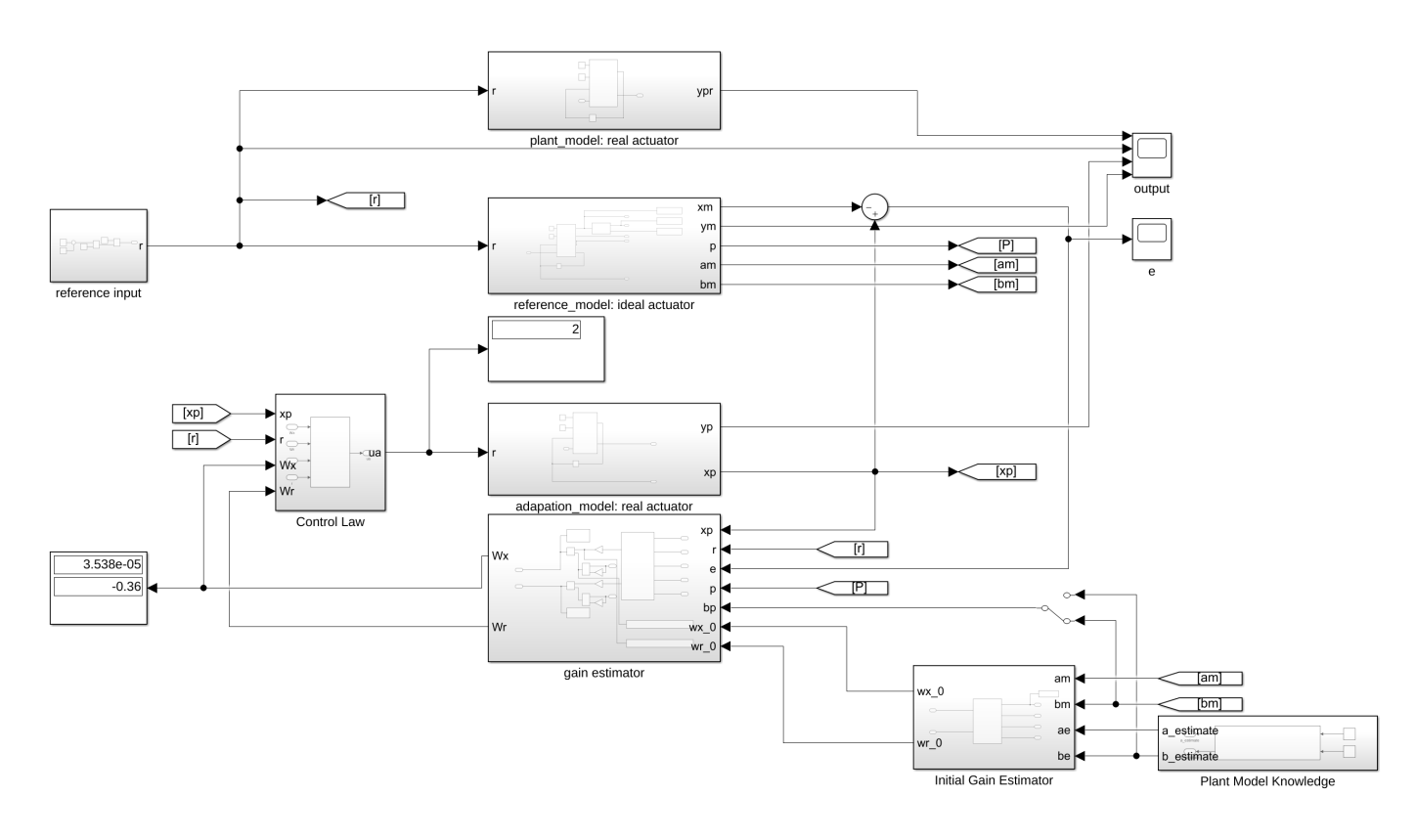
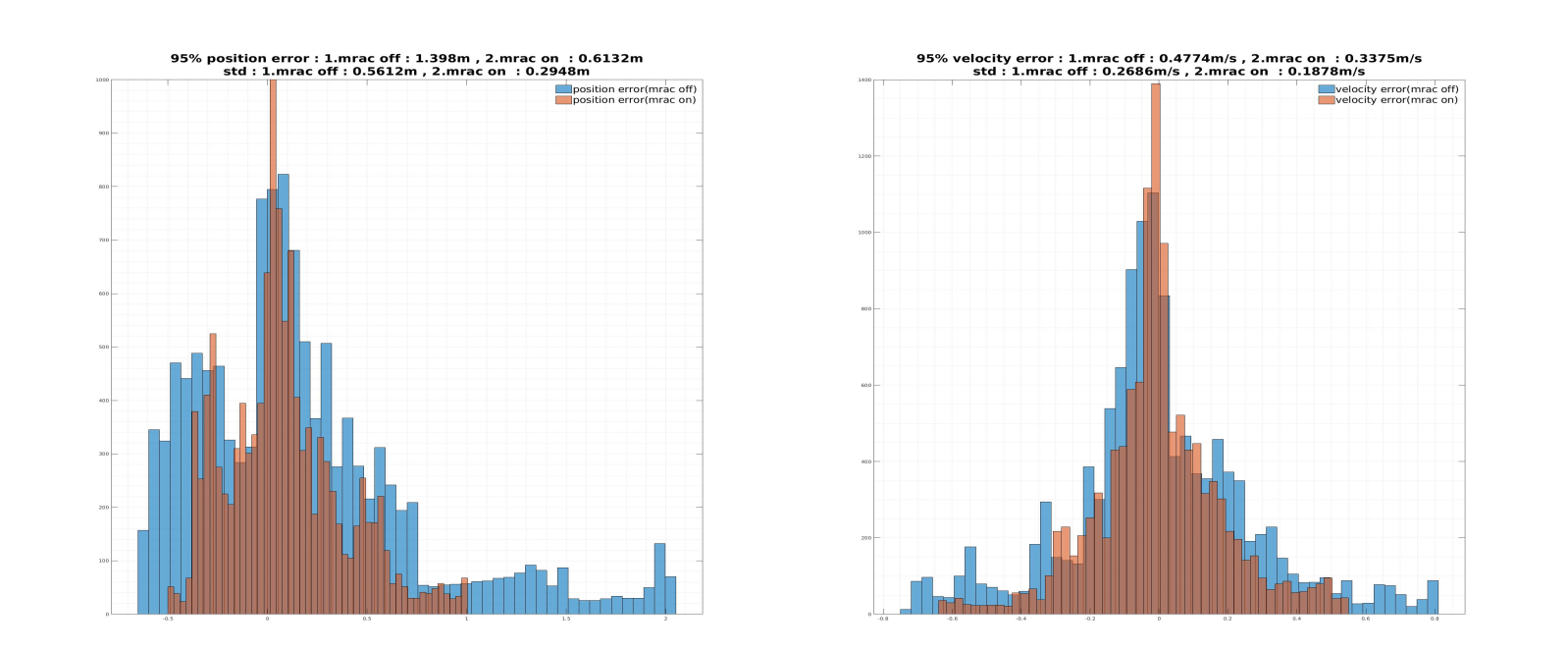
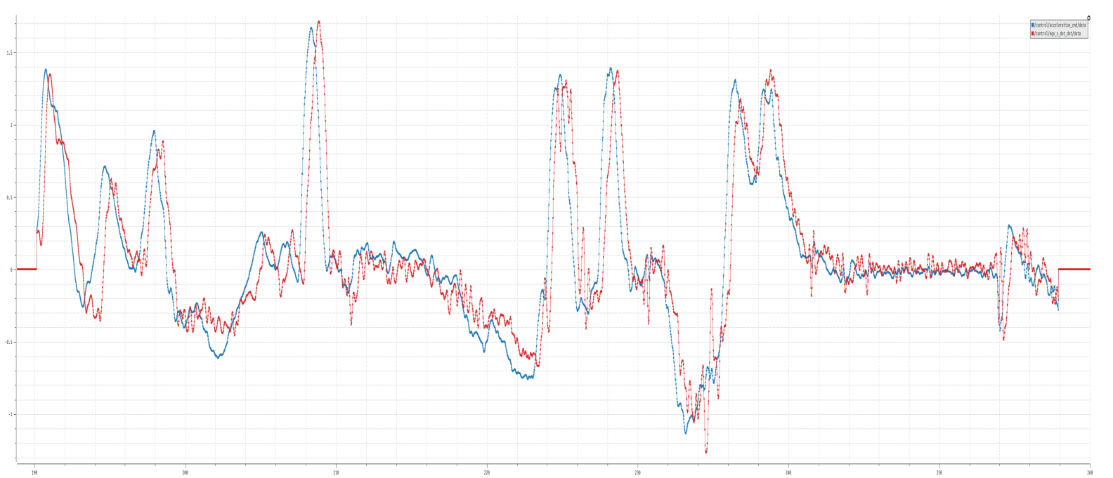
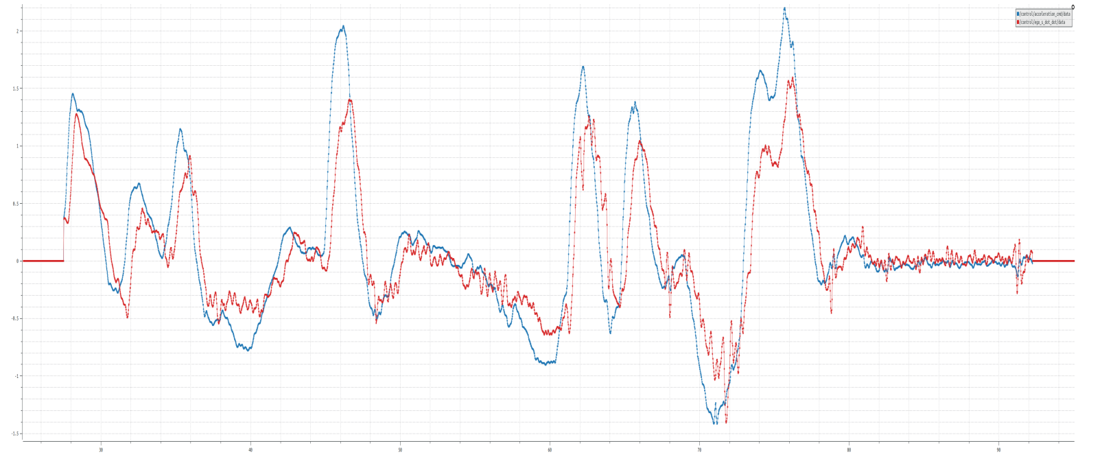
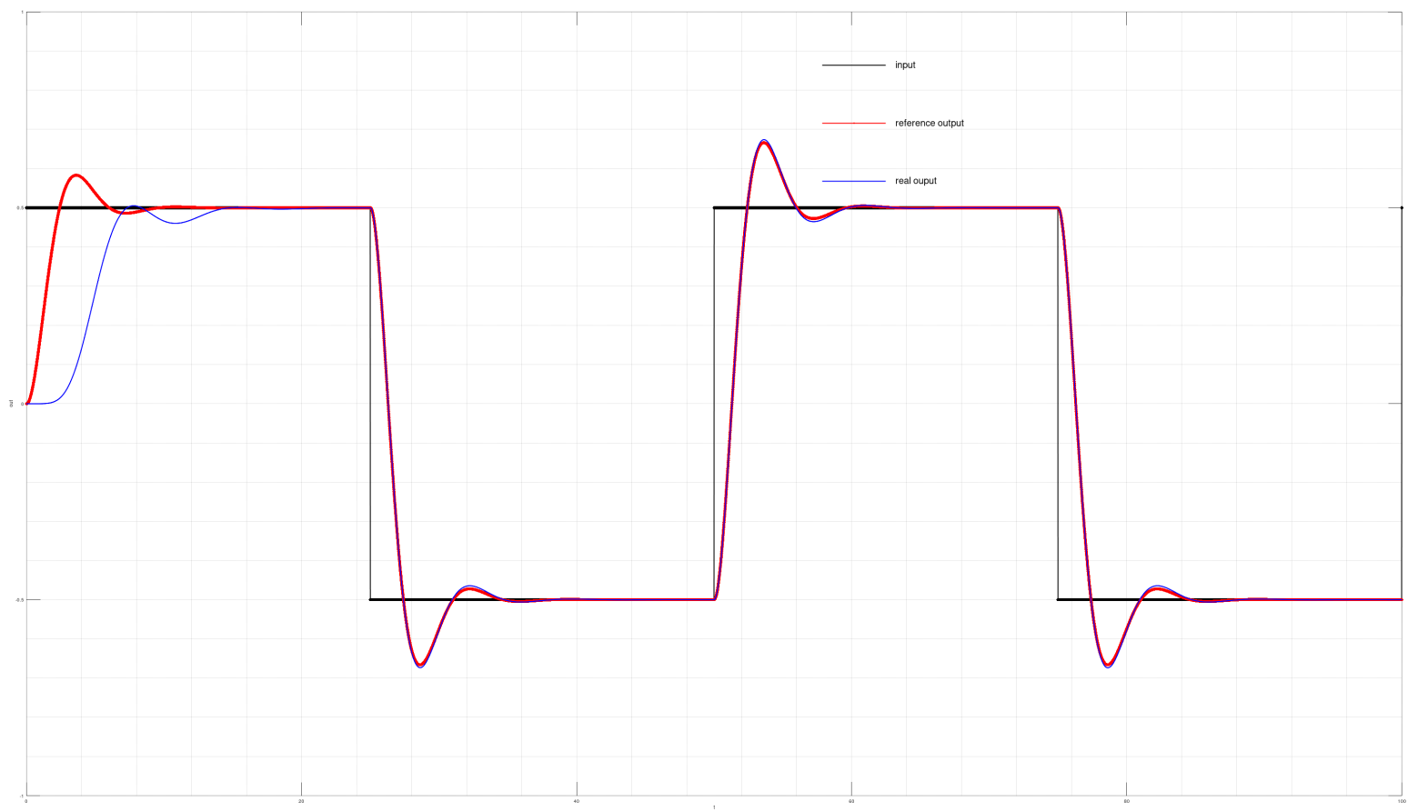
Performance