Model Predictive Control Part 2. Vehicle Lateral Dynamic Model

Motivation

First of all, we must ask: Why do we need to establish a dynamic model for vehicle lateral control? Simply put, when a vehicle operates at higher speeds, the assumption in kinematic models (such as the bicycle model) that “The direction of tire velocity aligns with the vehicle’s orientation” no longer holds. With centripetal force increasing quadratically with speed, the total lateral force acting on the vehicle become significant. Therefore, the introduction of a dynamic model aims to establish higher-order connections to better describe the non-linear characteristics of vehicle.

Model Assumptions

To simplify the model while maintaining generality, the dynamic model is built upon the following assumptions:

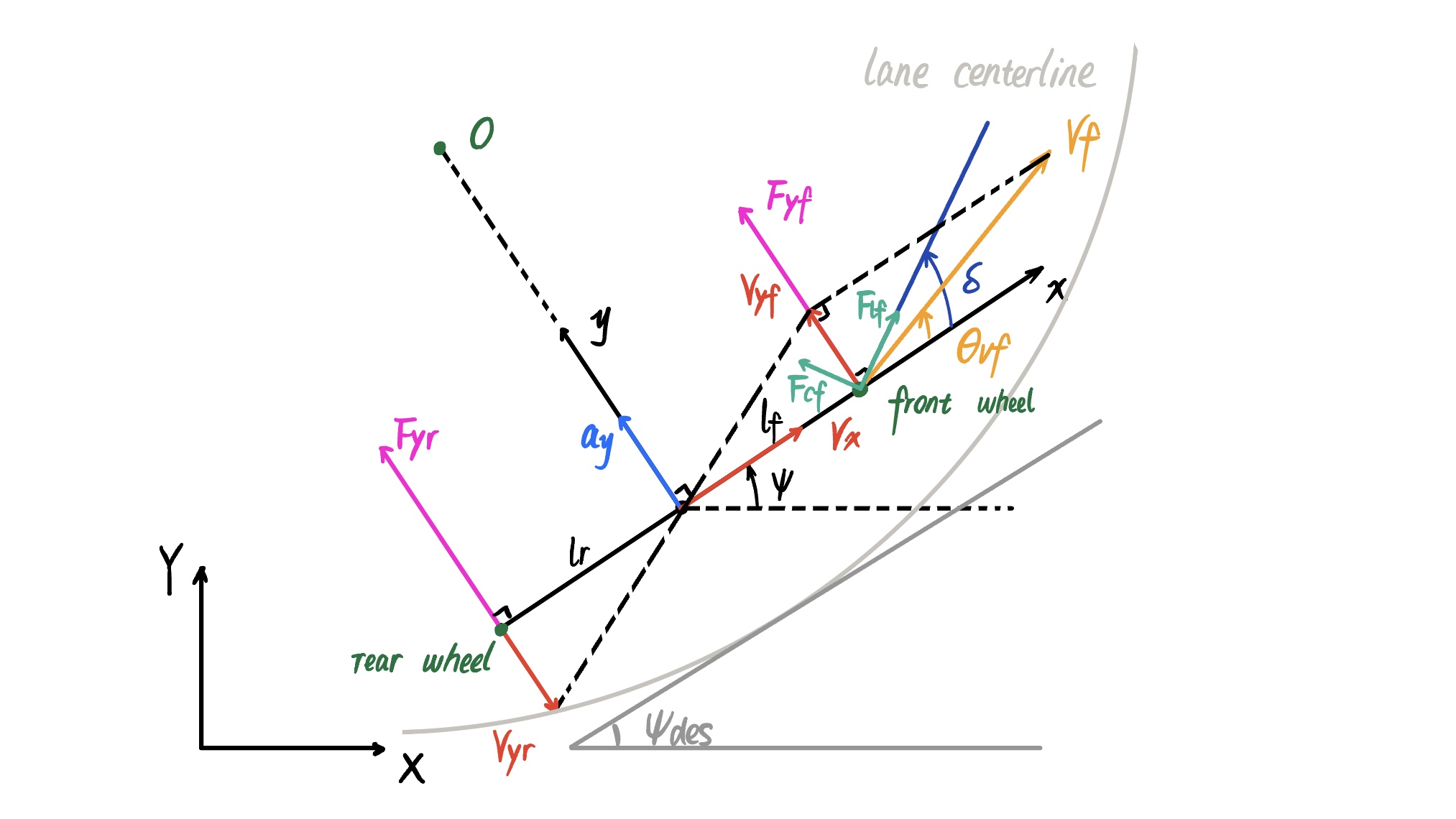
1.The angle between the tire velocity direction and the vehicle’s longitudinal direction denoted as $\theta_v$ (referred to as tire velocity angle) is small and satisfies the small angle assumption:

\[\theta_v \approx tan\theta_v\]

2.The angle between the tire steering angle $\delta$ and the tire velocity angle $\theta_v$ denoted as $\alpha$ (referred to as tire slip angle) is small.

3.The vehicle’s longitudinal velocity remains unchanged:

\[V_x : = Constant\]

4.Neglecting the influence of road banking angles $\phi$ on vehicle.

Coordinate System

This model is established under the Front-Left-Universe (FLU) inertial coordinate system. The origin of the coordinate system is fixed at the vehicle’s center of mass, with the $x$-axis pointing in the vehicle’s longitudinal direction towards the front. The $y$-axis is perpendicular to the $x$-axis and points to the left of the vehicle, while the $z$-axis is perpendicular to both the $x$ and $y$ axes, pointing upwards. It’s worth noting that the global (map) coordinate system is the East-North-Universe (ENU). The coordinate system is shown in sketch below

Force Analysis

According to Newton’s second law, the force in the $y$ direction (vehicle’s lateral) could be expressed as

\[F_{yf} + F_{yr} = ma_y\]

where $F_{yf}$ and $F_{yr}$ are the forces acting on the vehicle’s front and rear tires in the $y$ direction respectively, $m$ is the mass of vehicle, and $a_y$ is the vehicle’s acceleration in the $y$ direction.

The vehicle’s acceleration in the $y$ direction consists of two parts:

1. The acceleration caused by the movement of the vehicle in the $y$ direction, denoted as $\ddot{y}$
2. The centripetal acceleration of the vehicle, denoted as $a_{yc}$

\[a_y = \ddot{y}+a_{yc} = \ddot{y}+\omega^2R = \ddot{y}+\dot{\psi}^2R =\ddot{y}+V_x\dot{\psi}\]

Substituting $a_y$ back to lateral force equation, we have

\[F_{yf} + F{yr} = m(\ddot{y}+V_x\dot{\psi})\]

For the yaw dynamics analysis along the $z$-axis, torque balance yields:

\[I_z\ddot{\psi}=l_fF_{yf} - l_rF_{yr}\]

where $l_f$ and $l_r$ are the distances from the vehicle’s center of mass to the front and rear wheels, respectively.

Next, let’s analyze the lateral forces $F_{yf}$ and $F_{yr}$. Experimental evidence suggests that when the tire slip angle $\alpha$ is small, the magnitude of lateral force on the tire is proportional to the tire slip angle. The tire slip angle is defined as the angle between the tire’s steering angle and the tire velocity angle.

Therefore, the slip angle of the front wheels (steering wheels) $\alpha_f$ is given by

\[\alpha_f = \delta - \theta_{vf}\]

where $\delta$ is the front wheel steering angle and $\theta_{vf}$ is the front wheel velocity angle

Similarly, for the rear wheels (assuming they cannot steer), the slip angle is:

\[\alpha_r = 0 - \theta_{vr} = - \theta_{vr}\]

where $\theta_{vr}$ is the rear wheel velocity angle

Based on these points, the lateral tire forces can be rewritten as follows:

\[\begin{aligned} &F_{yf} = 2C_{\alpha_f}(\delta - \theta_{vf}) \\ &F_{yr} = -2C_{\alpha_r}\theta_{vr} \end{aligned}\]

where $C_{\alpha_f}$ and $C_{\alpha_r}$ are the lateral stiffness coefficients for the front and rear wheels, respectively

Using the small angle assumption and the kinematic equations, we have:

\[\begin{aligned} &\theta_{vf} \approx tan(\theta_{vf}) = \frac{\dot{y} + l_f\dot{\psi}}{V_x} \\ &\theta_{vr} \approx tan(\theta_{vr}) = \frac{\dot{y} - l_r\dot{\psi}}{V_x} \end{aligned}\]

Rearange the equation

\[\begin{aligned} &\ddot{y} = \frac{2}{m}[C_{\alpha_f}\delta - \frac{C_{\alpha_f}+C_{\alpha_r}}{V_x}\dot{y}+ \frac{-C_{\alpha_f}l_f+C_{\alpha_r}l_r}{V_x}\dot{\psi}] -V_x\dot{\psi} \\ &\ddot{\psi}=\frac{2}{I_z}(C_{\alpha_f}l_f\delta-\frac{C_{\alpha_f}l_f- C_{\alpha_r}l_r}{V_x}\dot{y}-\frac{C_{\alpha_f}l_f^2+C_{\alpha_r}l_r^2}{V_x}\dot{\psi}) \end{aligned}\]

Rewrite the above equation into matrix form

\[\begin{bmatrix} \dot{y} \\ \ddot{y} \\ \dot{\psi} \\ \ddot{\psi} \\ \end{bmatrix} = \begin{bmatrix} 0 & 1 & 0 & 0 \\ 0 & -\frac{2(C_{\alpha_f}+C_{\alpha_r})}{mV_x} & 0 & \frac{2(-C_{\alpha_f}l_f+C_{\alpha_r}l_r)}{mV_x}-V_x \\ 0 & 0 & 0 & 1 \\ 0 & -\frac{2(C_{\alpha_f}l_f- C_{\alpha_r}l_r)}{I_zV_x} & 0 & -\frac{2(C_{\alpha_f}l_f^2+C_{\alpha_r}l_r^2)}{I_zV_x} \\ \end{bmatrix} \begin{bmatrix} y \\ \dot{y} \\ \psi \\ \dot{\psi} \\ \end{bmatrix} + \begin{bmatrix} 0 \\ \frac{2C_{\alpha_f}}{m} \\ 0 \\ \frac{2C_{\alpha_f}l_f}{I_z} \\ \end{bmatrix} \delta\]

Error Dynamic Model

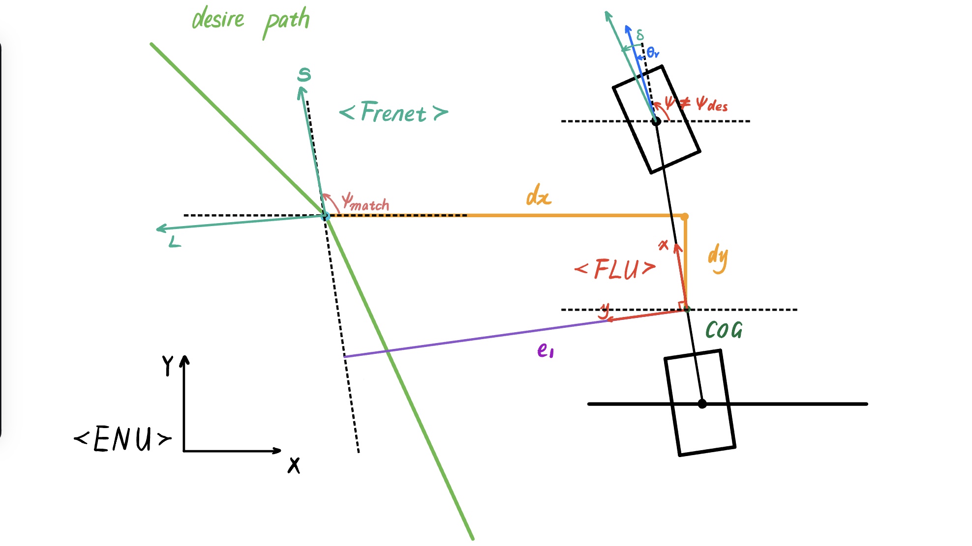
Setting the state variables in the dynamic model as errors will facilitate the design of subsequent feedback controllers. Therefore, define error state variables as follows:

\[\begin{aligned} e_1 &:= y-y_{des} \quad\text{lateral error} \\ e_2 &:= \psi-\psi_{des} \quad\text{front wheel heading error} \\ \end{aligned}\]

The ideal yaw rate is given by:

\[\dot{\psi}_{des} = \frac{V_x}{R}\]

The ideal lateral acceleration is:

\[a_{y_{des}} = \ddot{y}_{des}+a_{yc_{des}} = 0+\frac{V^2_x}{R} = V_x\dot{\psi}_{des}\]

Therefore, the lateral error $e_1$ can be rewritten as:

\[\ddot{e}_1 = a_y - a_{y_{des}} = \ddot{y}+V_x\dot{\psi}-V_x\dot{\psi}_{des} = \ddot{y}+V_x(\dot{\psi}-\dot{\psi}_{des}) = \ddot{y}+V_x\dot{e}_2\]

Since $V_x$ is constant, integrating the above equation yields:

\[\dot{e}_1 = \dot{y}+V_x(\psi-\psi_{des}) = \dot{y}+V_xe_2\]

From above, we obtain that

\[\begin{aligned} & \dot{y} = \dot{e}_1 - V_xe_2\\ & \ddot{y} = \ddot{e}_1 - V_x\dot{e}_2 \\ & \dot{\psi}= \dot{\psi}_{des}+\dot{e}_2 \\ \end{aligned}\]

Substituting above variables into the equations, we can get

\[\begin{aligned} &(\ddot{e}_1 - V_x\dot{e}_2) = \frac{2}{m}[C_{\alpha_f}\delta - \frac{C_{\alpha_f}+C_{\alpha_r}}{V_x}(\dot{e}_1 - V_xe_2)+ \frac{-C_{\alpha_f}l_f+C_{\alpha_r}l_r}{V_x}(\dot{\psi}_{des}+\dot{e}_2)] -V_x(\dot{\psi}_{des}+\dot{e}_2) \\ &\ddot{\psi}=\frac{2}{I_z}(C_{\alpha_f}l_f\delta-\frac{C_{\alpha_f}l_f- C_{\alpha_r}l_r}{V_x}(\dot{e}_1 - V_xe_2)-\frac{C_{\alpha_f}l_f^2+C_{\alpha_r}l_r^2}{V_x}(\dot{\psi}_{des}+\dot{e}_2)) \end{aligned}\]

Rearange to simplify the equations

\[\begin{aligned} &\ddot{e}_1 = \frac{2C_{\alpha_f}}{m}\delta+\frac{-2(C_{\alpha_f}+C_{\alpha_r})}{mV_x}\dot{e}_1 +\frac{2(C_{\alpha_f}+C_{\alpha_r})}{m}e_2 + \frac{2(-C_{\alpha_f}l_f+C_{\alpha_r}l_r)}{mV_x}\dot{e}_2 +(\frac{2(-C_{\alpha_f}l_f+C_{\alpha_r}l_r)}{mV_x}-V_x)\dot{\psi}_{des} \\ &\ddot{\psi} = \frac{2C_{\alpha_f}l_f}{I_z}\delta+\frac{-2(C_{\alpha_f}l_f-C_{\alpha_r}l_r)}{I_zV_x}\dot{e}_1 +\frac{2(C_{\alpha_f}l_f-C_{\alpha_r}l_r)}{I_z}e_2 +\frac{-2(C_{\alpha_f}l^2_f+C_{\alpha_r}l^2_r)}{I_zV_x}\dot{e}_2 +\frac{-2(C_{\alpha_f}l^2_f+C_{\alpha_r}l^2_r)}{I_zV_x}\dot{\psi}_{des} \end{aligned}\]

Then rewrite the dynamics in matrix form

\[\begin{bmatrix} \dot{e}_1 \\ \ddot{e}_1 \\ \dot{e}_2 \\ \ddot{e}_2 \\ \end{bmatrix}= \begin{bmatrix} 0 & 1 & 0 & 0 \\ 0 & \frac{-2(C_{\alpha_f}+C_{\alpha_r})}{mV_x} & \frac{2(C_{\alpha_f}+C_{\alpha_r})}{m} & \frac{2(-C_{\alpha_f}l_f+C_{\alpha_r}l_r)}{mV_x}\\ 0 & 0 & 0 & 1 \\ 0 & \frac{-2(C_{\alpha_f}l_f-C_{\alpha_r}l_r)}{I_zV_x} & \frac{2(C_{\alpha_f}l_f-C_{\alpha_r}l_r)}{I_z} & \frac{-2(C_{\alpha_f}l^2_f+C_{\alpha_r}l^2_r)}{I_zV_x} \\ \end{bmatrix} \begin{bmatrix} e_1 \\ \dot{e}_1 \\ e_2 \\ \dot{e}_2 \\ \end{bmatrix} + \begin{bmatrix} 0 \\ \frac{2C_{\alpha_f}}{m} \\ 0 \\ \frac{2C_{\alpha_f}l_f}{I_z} \\ \end{bmatrix} \delta + \begin{bmatrix} 0 \\ \frac{2(-C_{\alpha_f}l_f+C_{\alpha_r}l_r)}{mV_x}-V_x \\ 0 \\ \frac{-2(C_{\alpha_f}l^2_f+C_{\alpha_r}l^2_r)}{I_zV_x} \\ \end{bmatrix} \dot{\psi}_{des}\]

Finally, the continuous-time error dynamics could be expressed as

\[\dot{x} = Ax + B\delta + B_c\dot{\psi}_{des}\]

where

\[\begin{aligned} x &= \begin{bmatrix} e_1 \\ \dot{e}_1 \\ e_2 \\ \dot{e}_2 \\ \end{bmatrix} \\ \\ A &= \begin{bmatrix} 0 & 1 & 0 & 0 \\ 0 & \frac{-2(C_{\alpha_f}+C_{\alpha_r})}{mV_x} & \frac{2(C_{\alpha_f}+C_{\alpha_r})}{m} & \frac{2(-C_{\alpha_f}l_f+C_{\alpha_r}l_r)}{mV_x}\\ 0 & 0 & 0 & 1 \\ 0 & \frac{-2(C_{\alpha_f}l_f-C_{\alpha_r}l_r)}{I_zV_x} & \frac{2(C_{\alpha_f}l_f-C_{\alpha_r}l_r)}{I_z} & \frac{-2(C_{\alpha_f}l^2_f+C_{\alpha_r}l^2_r)}{I_zV_x} \\ \end{bmatrix} \\ \\ B &= \begin{bmatrix} 0 \\ \frac{2C_{\alpha_f}}{m} \\ 0 \\ \frac{2C_{\alpha_f}l_f}{I_z} \\ \end{bmatrix} \\ \\ B_c &= \begin{bmatrix} 0 \\ \frac{2(-C_{\alpha_f}l_f+C_{\alpha_r}l_r)}{mV_x}-V_x \\ 0 \\ \frac{-2(C_{\alpha_f}l^2_f+C_{\alpha_r}l^2_r)}{I_zV_x} \\ \end{bmatrix} \end{aligned}\]

This model represents the error dynamics of the lateral position, lateral velocity, front-wheel heading angle, and angular velocity errors. It provides a foundation for designing controllers to regulate the vehicle’s lateral motion.