Linear Quadratic Optimal Tracking For Time Varying Non-linear System
Motivation
Tracking a desired trajectory while minimizing a quadratic cost function is a critical problem in many engineering and scientific domains. However, solving this problem analytically can be challenging, especially when dealing with time-varying systems. In this post, we present a comprehensive framework for deriving the analytical solution to the generalized tracking problem with quadratic cost for a time-varying system. We provide a detailed description of the problem formulation and the optimal policy derivation process, covering both continuous and discrete time cases. Our approach offers a valueable tool for tackling real-world tracking tasks and advancing our understanding of control strategies for dynamic systems.
System Linearization
Consider a time-varying non-linear dynamical system
\[\dot x = f(t,x,u)\]we approximate the system with a first-order Taylor expansion at $ (x_0,u_0)$ , then
\[\begin{aligned} \dot x &= f(t,x_0,u_0) + \frac{\partial f(t,x_0,u_0)}{\partial x}(x - x_0) + \frac{\partial f(t,x_0,u_0)}{\partial u}(u - u_0) \\ &= \frac{\partial f(t,x_0,u_0)}{\partial x} x + \frac{\partial f(t,x_0,u_0)}{\partial u}u + [f(t,x_0,u_0) - \frac{\partial f(t,x_0,u_0)}{\partial x}x_0-\frac{\partial f(t,x_0,u_0)}{\partial u}u_0] \end{aligned}\]rewrite the linear time-varying affine of original system in state space form
\[\dot x = A(t)x + B(t)u + c(t)\]where
\[\begin{aligned} A(t) &= \frac{\partial f(t,x_0,u_0)}{\partial x} \\ B(t) &= \frac{\partial f(t,x_0,u_0)}{\partial u} \\ c(t) &= f(t,x_0,u_0) - \frac{\partial f(t,x_0,u_0)}{\partial x}x_0-\frac{\partial f(t,x_0,u_0)}{\partial u}u_0 \end{aligned}\]Cost Design
The general instantaneous cost (running cost function) $l$ could be expressed as
\[l(t,x,u) = x^TQ_{xx}x + u^TR_{uu}u + 2x^TNu + 2q_x^Tx + 2r_u^Tu+q_0+r_0\]rewrite it in quadratic form
\[l(t,x,u) = \begin{bmatrix} x \\ 1 \end{bmatrix}^TQ(t)\begin{bmatrix} x \\ 1 \end{bmatrix} + \begin{bmatrix} u \\ 1 \end{bmatrix}^TR(t)\begin{bmatrix} u \\ 1 \end{bmatrix} + 2 x^TN(t)u\]for all $t \in [t,t_f]$
\[\begin{aligned} Q(t) &= \begin{bmatrix} Q_{xx}(t) & q_x(t) \\ q_x^T(t) & q_0(t)\end{bmatrix},Q_{xx}(t) \succ 0 \\ R(t) &= \begin{bmatrix} R_{uu}(t) & r_u(t) \\ r_u^T(t) & r_0(t)\end{bmatrix},R_{uu}(t) \succeq 0 \end{aligned}\]Consider a ‘optimal tracking’ problem, the running cost function could be designed as
\[\begin{aligned} l(t,x,u) = &(x - x_r(t))^TQ_t(t)(x-x_r(t)) + (u-u_r(t))^TR_t(t)(u-u_r(t)) + 2(x-x_r(t))^TN_t(t)(u-u_r(t)) \\ =&x^TQ_t(t)x+u^TR_t(t)u+2x^TN_t(t)u \\ &+2(-Q_t(t)x_r-N_t(t)u_r)^Tx+2(-R_t(t)u_r-N_t^T(t)x_r)^Tu \\ &+x_r^TQ_t(t)x_r + u_r^TR_t(t)u_r + 2x_r^TN_t(t)u_r \end{aligned}\]by fitting the instantaneous cost in general quadratic form, we have
\[\begin{aligned} Q_{xx} &= Q_t\\ R_{uu} &= R_t\\ N &= N_t \\ q_x &= -Q_tx_r-N_tu_r \\ r_u &= -R_tu_r-N_t^Tx_r \\ q_0 &= x_r^TQ_tx_r + 2x_r^TN_tu_r \\ r_0 &= u_r^TR_tu_r\\ \end{aligned}\]the partial derivative of instantaneous cost $l$ with respect to input $u$ is
\[\frac{\partial l}{\partial u} = 2(R_tu+N_t^Tx-Q_tu_r-N_t^Tx_r)\]the total cost function is given by
\[J(t,x,u) = \int_{t}^{t_f} l(s,x,u) ds + l_f(t_f,x,u)\]Derivation of Optimal Solution
Guess a general solution of optimal cost is
\[J^{\ast}(t,x) = x^TP_{xx}(t)x + 2p_x^T(t)x+p_0(t), P_{xx}(t) = P_{xx}^T(t) \succ 0\]rewrite it in quadratic form
\[J^{\ast} (t,x) = \begin{bmatrix} x \\ 1 \end{bmatrix}^TP(t)\begin{bmatrix} x \\ 1 \end{bmatrix}\]for all $t \in [t,t_f]$
\[P(t) = \begin{bmatrix} P_{xx}(t) & p_x(t)\\ p_x^T(t) & p_0(t)\end{bmatrix},P_{xx}(t) \succ 0\]In this case, the partial derivative of the optimal cost function is
\[\begin{aligned} & \frac{\partial J^{\ast}}{\partial x} = 2P_{xx}(t)x+2p_x(t)\\ & \frac{\partial J^{\ast}}{\partial t} = x^T\dot P_{xx}(t)x + 2\dot p_x^T(t)x+\dot p_0(t) \end{aligned}\]The HJB equation states the necessary and sufficient condition for optimality as
\[\inf_{u[t,t+\Delta t] } l(t,x(t),u(t)) + V_t(t,x) + V_x(t,x)f(t,x,u(t)) = 0\]where the value function(optimal cost to go) $V$ is defined as
\[V(t,x) = \inf_{u[t,t_f]}J(t,x,u) = J^{\ast}(t,x)\]Substitute the solution in HJB
\[\begin{aligned} &\min_{u[t,t+\Delta t]}[l(t,x,u) + \frac{\partial J^{\ast}}{\partial t} + \frac{\partial J^{\ast}}{\partial x}\lbrack A(t)x+B(t)u+c(t)) \rbrack = 0 \\ &\min_{u[t,t+\Delta t]}[l(t,x,u)+ x^T\dot P_{xx}(t)x + 2\dot p_x^T(t)x+\dot p_0(t)+2(P_{xx}(t)x+p_x(t))^T\lbrack A(t)x+B(t)u+c(t) \rbrack = 0 \end{aligned}\]then the optimal $u^{\ast}$ must satisfy the condition
\[\begin{aligned} & \frac{\partial}{\partial u} = \frac{\partial l}{\partial u} + 2B^T(P_{xx}(t)x+p_x(t)) = 0 \\ & \frac{\partial}{\partial u} = 2(R_tu^{\ast}+N_t^Tx-R_tu_r-N_t^Tx_r+B^TP_{xx}(t)x+B^Tp_x(t)) = 0 \\ \\ -R_tu^{\ast} &= (N_t^T + B^TP_{xx})x+(B^Tp_x-R_tu_r-N_t^Tx_r)\\ u^{\ast}(t) &= - R_t^{-1}(N_t^T + B^TP_{xx})x - R_t^{-1}(B^Tp_x-R_tu_r-N_t^Tx_r) \\ &= Kx+k \end{aligned}\]Inserting the optimal $u^{\ast}$ to HJB equation
\[\begin{aligned} 0 &= l+x^T\dot P_{xx}x+2\dot p_x^Tx+\dot p_0+2(P_{xx}x+p_x)^T[Ax+Bu+c] \\ &= x^TQ_tx+u^TR_tu+2x^TN_tu+x_r^TQ_tx_r+u_r^TR_tu_r+2x_r^TN_tu_r-2(Q_tx_r+N_tu_r)^Tx-2(R_tu_r+N_t^Tx_r)^T(Kx+k)+x^T\dot P_{xx}x+2\dot p_x^Tx+\dot p_0+2(P_{xx}x+p_x)^T[Ax+B(Kx+k)+c]\\ &= x^TQ_tx+(Kx+k)^TR_t(Kx+k)+2x^TN_t(Kx+k)+x_r^TQ_tx_r+u_r^TR_tu_r+2x_r^TN_tu_r-2(Q_tx_r+N_tu_r)^Tx-2(R_tu_r+N_t^Tx_r)^T(Kx+k)+x^T\dot P_{xx}x+2\dot p_x^Tx+\dot p_0+2(P_{xx}x+p_x)^T[(A+BK)x+Bk+c]\\ \\ -x^T\dot P_{xx}x-2\dot p_x^Tx-\dot p_0 &= x^TQ_tx+x^TK^TR_tKx+2k^TR_tKx+k^TR_tk+2x^TN_tKx+2x^TN_tk+x_r^TQ_tx_r+u_r^TR_tu_r+2x_r^TN_tu_r-2(Q_tx_r+N_tu_r)^Tx-2(R_tu_r+N_t^Tx_r)^TKx-2(R_tu_r+N_t^Tx_r)^Tk+2x^TP_{xx}(A+BK)x+2x^TP_{xx}(Bk+c)+2p_x^T(A+BK)x+2p_x^T(Bk+c)\\ &= x^T(Q_t+K^TR_tK+2N_tK+2P_{xx}A+2P_{xx}BK)x\\ & \qquad +2(K^TR_tk+N_tk-N_tu_r-Q_tx_r-K^TR_tu_r-K^TN_t^Tx_r+(A+BK)^Tp_x+P_{xx}(Bk+c))^Tx\\ & \qquad +k^TR_tk+x_r^TQ_tx_r+u_r^TR_tu_r+2x_r^TN_tu_r-2(R_tu_r+N_t^Tx_r)^Tk+2p_x^T(Bk+c)\\ \end{aligned}\]Collect quadratic, linear and offset terms and set them each individually equal to zero, yielding
\[\begin{aligned} -\dot P_{xx} &= Q_t+K^TR_tK+2N_tK+2P_{xx}A+2P_{xx}BK \\ & = Q_t+(P_{xx}B+N_t)R_t^{-1}(P_{xx}B+N_t)^T-2(P_{xx}B+N_t)R_t^{-1}(P_{xx}B+N_t)^T+2P_{xx}A\\ & = Q_t-(P_{xx}B+N_t)R_t^{-1}(P_{xx}B+N_t)^T+P_{xx}A+A^TP_{xx}\\ \\ -\dot p_x &= K^TR_tk+N_tk-N_tu_r-Q_tx_r-K^TR_tu_r-K^TN_t^Tx_r+(A+BK)^Tp_x+P_{xx}(Bk+c) \\ & = (P_{xx}B+N_t)R_t^{-1}(B^Tp_x+r_t)-(N_tu_r+Q_tx_r)+N_tk-K^T(R_tu_r+N_t^Tx_r)+K^TB^Tp_x+A^Tp_x+P_{xx}Bk+P_{xx}c \\ & = (P_{xx}B+N_t)R_t^{-1}(B^Tp_x+r_t)-(N_tu_r+Q_tx_r)+(N_t+P_{xx}B)k-K^T(R_tu_r+N_t^Tx_r-B^Tp_x)+A^Tp_x+P_{xx}c \\ & = (P_{xx}B+N_t)R_t^{-1}(B^Tp_x+r_t)-(N_tu_r+Q_tx_r)-(N_t+P_{xx}B)R_t^{-1}(B^Tp_x+r_t)+(P_{xx}B+N_t)R_t^{-1}(R_tu_r+N_t^Tx_r-B^Tp_x)+A^Tp_x+P_{xx}c \\ & = (P_{xx}B+N_t)R_t^{-1}(B^Tp_x+r_t)-(N_tu_r+Q_tx_r)-(N_t+P_{xx}B)R_t^{-1}(B^Tp_x+r_t)-(P_{xx}B+N_t)R_t^{-1}(B^Tp_x+r_t)+A^Tp_x+P_{xx}c \\ & = -N_tu_r-Q_tx_r-(N_t+P_{xx}B)R_t^{-1}(B^Tp_x+r_t)+A^Tp_x+P_{xx}c\\ \\ -\dot p_0 &= k^TR_tk+x_r^TQ_tx_r+u_r^TR_tu_r+2x_r^TN_tu_r-2(R_tu_r+N_t^Tx_r)^Tk+2p_x^T(Bk+c) \\ & = (r_t+B^Tp_x)^TR_t^{-1}(r_t+B^Tp_x)+x_r^TQ_tx_r+u_r^TR_tu_r+2x_r^TN_tu_r+2(R_tu_r+N_t^Tx_r)^TR_t^{-1}(B^Tp_x+r_t)-2p_x^TBR_t^{-1}(B^Tp_x+r_t)+2p_x^Tc\\ & = x_r^TQ_tx_r+u_r^TR_tu_r+2x_r^TN_tu_r + (B^Tp_x+r_t+2R_tu_r+2N_t^Tx_r-2B^Tp_x)^TR_t^{-1}(r_t+B^Tp_x)+2p_x^Tc\\ & = x_r^TQ_tx_r+u_r^TR_tu_r+2x_r^TN_tu_r - (r_t+B^Tp_x)^TR_t^{-1}(r_t+B^Tp_x)+2p_x^Tc \end{aligned}\]Summary
The continuous differential riccati equations are
\[\begin{aligned} -\dot P_{xx} &= Q_t-(P_{xx}B+N_t)R_t^{-1}(P_{xx}B+N_t)^T+P_{xx}A+A^TP_{xx} \\ -\dot p_x &= -N_tu_r-Q_tx_r-(N_t+P_{xx}B)R_t^{-1}(B^Tp_x+r_t)+A^Tp_x+P_{xx}c \\ -\dot p_0 &= x_r^TQ_tx_r+u_r^TR_tu_r+2x_r^TN_tu_r - (r_t+B^Tp_x)^TR_t^{-1}(r_t+B^Tp_x)+2p_x^Tc\\ \\ u^{\ast} &= Kx+k \\ K &= - R_t^{-1}(N_t^T + B^TP_{xx}) \\ k &= - R_t^{-1}(B^Tp_x-R_tu_r-N_t^Tx_r) \end{aligned}\]Linear Optimal Tracking in Discrete Time
Consider a discrete-time time-varying linear system:
\[x_{k+1} = A_d(k)x_k+B_d(k)u_k+c_d(k)\]the system could be discretized from the linear time-varying continuous system in previous section.
For tracking problems, a general instantaneous cost could be expressed as
\[\begin{aligned} l_k(x_k,u_k) =& (x_k - x_{r_k})^TQ_k(x_k - x_{r_k}) + (u_k - u_{r_k})^TR_k(u_k - u_{r_k}) + 2(x_k-x_{r_k})^TN_k(u_k-u_{r_k}) \\ =&x_k^TQ_kx_k+u_k^TR_ku_k+2x_k^TN_ku_k \\ &+2(-Q_kx_{r_k}-N_ku_{r_k})^Tx_k+2(-R_ku_{r_k}-N_k^Tx_{r_k})^Tu_k \\ &+x_{r_k}^TQ_kx_{r_k} + u_{r_k}^TR_ku_{r_k} + 2x_{r_k}^TN_ku_{r_k} \\ \end{aligned}\]rewrite in compact form
\[\begin{aligned} l_k(x_k,u_k) &= \begin{bmatrix} x_k^T & u_k^T\end{bmatrix}\begin{bmatrix}D_{xx} & D_{xu} \\ D_{ux} & D_{uu}\end{bmatrix}\begin{bmatrix}x_k \\u_k \end{bmatrix}+2\begin{bmatrix}d_x^T & d_u^T\end{bmatrix}\begin{bmatrix}x_k \\u_k \end{bmatrix}+d_{0_k} \\ &=x_k^TD_{xx}x_k+u_k^TD_{uu}u_k+2x_k^TD_{xu}u_k+2d_x^Tx_k+2d_u^Tu_k+d_{0_k} \end{aligned}\]comparing equations above, it’s easy to show that
\[\begin{aligned} D_{xx} &= Q_k \\ D_{uu} &= R_k \\ D_{xu} &= N_k \\ d_x &= -Q_kx_{r_k}-N_ku_{r_k}\\ d_u &= -R_ku_{r_k}-N_k^Tx_{r_k}\\ d_{0_k} &= x_{r_k}^TQ_kx_{r_k} + u_{r_k}^TR_ku_{r_k} + 2x_{r_k}^TN_ku_{r_k} \end{aligned}\]define
\[\begin{aligned} \xi_k &= \begin{bmatrix} x_k \\ u_k \end{bmatrix} \\ D_k &= \begin{bmatrix} Q_k & N_k \\ N_k^T & R_k \end{bmatrix} \\ d_k &= \begin{bmatrix} -Q_kx_{r_k}-N_ku_{r_k}\\ -R_ku_{r_k}-N_k^Tx_{r_k}\end{bmatrix} \\ \end{aligned}\]the instantaneous cost at time stamp $t_k$ could be further simplified to a quadratic function of augment state $\xi_k$
\[\begin{aligned} l_k(x_k,u_k) &= x_k^TD_{xx}x_k+u_k^TD_{uu}u_k+2x_k^TD_{xu}u_k+2d_x^Tx_k+2d_u^Tu_k+d_{0_k} \\ &= \xi_k^TD_k\xi_k + 2d_k^T\xi_k+d_{0_k} \end{aligned}\]Inductive Step
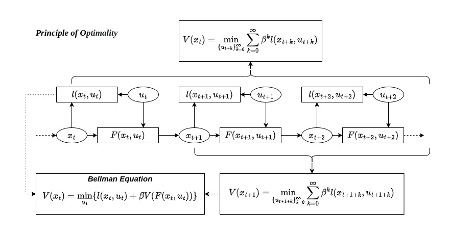
The total cost $J(x_K,u)$ is defined as
\[\begin{aligned} J_k(x_k,U) = l_f(x_N,u_N)+ \sum_{i=k}^{N-1}l_i(x_i,u_i) \end{aligned}\]The value function (optimal cost to go) $V_k(x_k)$ is defined as
\[\begin{aligned} V_N(x_N) &= l_f(x_N,u_N)\\ V_k(x_k) &= J_k^{\ast}(x_k,U^{\ast})\\ &= \inf_UJ(x_k,U) \\ &= l_f(x_N,u_N)+\inf_{U}\sum_{i=k}^{N-1}l_i(x_i,u_i)\\ &= l_k(x_k,u_k^{\ast}) + l_f(x_N,u_N)+\inf_{U^{-}}\sum_{i=k+1}^{N-1}l_i(x_i,u_i)\\ &= l_k(x_k,u_k^{\ast}) + V_{k+1}(x_{k+1})\\ &= \inf_{u_k}[\ l_k(x_k,u_k)+V_{k+1}(x_{k+1})\ ] \\ &= \inf_{u_k}[\ l_k(x_k,u_k)+V_{k+1}(f_d(x_k,u_k))\ ] \end{aligned}\]Next, for each time stamp $t_k$, q-function(reinforcement learning) could be defined as
\[\begin{aligned} q_k(x_k,u_k) = \left\{ \begin{array}{ll} \ l_f(x_N,u_N) & \mbox{k = N} \\ \ l_k(x_k,u_k) + \inf_{u_{k+1}}q_{k+1}(x_{k+1},u_{k+1}) & \mbox{k < N}\\ \ = l_k(x_k,u_k) + V_{k+1}(x_{k+1}) \end{array} \right. \end{aligned}\]the inductive hypothesis that q-function and value function has the form
\[\begin{aligned} q_k(x_k,u_k) &= \xi_k^TP_k\xi_k+2p_k^T\xi_k+p_{0_k} \\ V_k(x_k) &= x_k^TZ_kx_k + 2z_k^Tx_k+z_{0_k} \end{aligned}\]base case at $k = N(t = t_f)$ , the terminal value function could be perfectly fitted in above form
\[\begin{aligned} q_N(x_N,u_N) &= l_f(x_N,u_N) \\ &= \xi_N^TD_N\xi_N+2d_N^T\xi_N+d_{0_N}\\ &= \xi_N^TP_N\xi_N+2p_N^T\xi_N+p_{0_N} \end{aligned}\]where
\[\begin{aligned} P_N &= D_N \\ p_N &= d_N \\ p_{0_N} &= d_{0_N} \end{aligned}\]For $\forall t \in [t_k, t_{N-1}]$ , suppose minimum solution is feasible, we have
\[\begin{aligned} q_k(x_k,u_k) &= l_k(x_k,u_k) + V_{k+1}(x_{k+1}) \\ \xi_k^TP_k\xi_k+2p_k^T\xi_k+p_{0_k} &= \xi_k^TD_k\xi_k + 2d_k^T\xi_k+d_{0_k} + V_{k+1}(x_{k+1}) \\ \end{aligned}\]compute $V_{k+1}(x_{k+1})$
\[\begin{aligned} V_{k+1}(x_{k+1}) &= {x_{k+1}}^TZ_{k+1}x_{k+1} + 2z_{x_{k+1}}^Tx_{k+1} + z_{0_{k+1}}\\ &=(A_dx_k+B_du_k+C_d)^TZ_{k+1}(A_dx_k+B_du_k+C_d) + 2z_{x_{k+1}}^T(A_dx_k+B_du_k+C_d) + z_{0_{k+1}}\\ &\text{let $F_d = \begin{bmatrix} A_d & B_d \end{bmatrix}$, and ${\xi_k}^T = \begin{bmatrix} x_k^T & u_k^T \end{bmatrix}$} \\ &= (F_d\xi_k+C_d)^TZ_{k+1}(F_d\xi_k+C_d)+2z_{x_{k+1}}^T(F_d\xi_k+C_d)+z_{0_{k+1}}\\ &= {\xi_k}^TF_d^TZ_{k+1}F_d\xi_k+2(F_d^TZ_{k+1}C_d+F_d^Tz_{x_{k+1}})^T\xi_k+(C_d^TZ_{k+1}C_d+2z_{x_{k+1}}^TC_d+z_{0_{k+1}}) \end{aligned}\]substitute back to q-function, we have
\[\begin{aligned} \xi_k^TP_k\xi_k+2p_k^T\xi_k+p_{0_k} &= \xi_k^TD_k\xi_k + 2d_k^T\xi_k+d_{0_k} + V_{k+1}(x_{k+1}) \\ \xi_k^TP_k\xi_k+2p_k^T\xi_k+p_{0_k} &= \xi_k^TD_k\xi_k + 2d_k^T\xi_k+d_{0_k} + {\xi_k}^TF_d^TZ_{k+1}F_d\xi_d+2(F_d^TZ_{k+1}C_d+F_d^Tz_{x_{k+1}})^T\xi_k+z_{0_{k+1}}+2z_{x_{k+1}}^TC_d+C_dZ_{k+1}C_d\\ &= \xi_k^T(D_k+F_d^TZ_{k+1}F_d)\xi_k+2(d_k+F_d^TZ_{k+1}C_d+F_d^Tz_{x_{k+1}})^T\xi_k+(d_{0_k}+C_d^TZ_{k+1}C_d+2z_{x_{k+1}}^TC_d+z_{0_{k+1}}) \end{aligned}\]Collect quadratic, linear and offset terms
\[\begin{aligned} P_k &= D_k+F_d^TZ_{k+1}F_d \\ p_k &= d_k+F_d^TZ_{k+1}C_d+F_d^Tz_{x_{k+1}}\\ p_{0_k} &= d_{0_k}+C_d^TZ_{k+1}C_d+2z_{x_{k+1}}^TC_d+z_{0_{k+1}} \end{aligned}\]quadratic coefficient
\[\begin{aligned} P_k &= D_k+F_d^TZ_{k+1}F_d \\ P_k &= \begin{bmatrix} Q_k & N_k \\ N_k^T & R_k \end{bmatrix} + \begin{bmatrix}A_d^T\\B_d^T\end{bmatrix}Z_{k+1}\begin{bmatrix}A_d&B_d\end{bmatrix}\\ P_k &= \begin{bmatrix} Q_k & N_k \\ N_k^T & R_k \end{bmatrix} + \begin{bmatrix} A_d^TZ_{k+1}A_d & A_d^TZ_{k+1}B_d \\ B_d^TZ_{k+1}A_d & B_d^TZ_{k+1}B_d \end{bmatrix}\\ P_k &= \begin{bmatrix} Q_k+A_d^TZ_{k+1}A_d & N_k+A_d^TZ_{k+1}B_d \\ N_k^T+B_d^TZ_{k+1}A_d & R_k+B_d^TZ_{k+1}B_d \end{bmatrix}\\ \begin{bmatrix} P_{xx} & P_{xu} \\ P_{xu}^T & P_{uu} \end{bmatrix} &= \begin{bmatrix} Q_k+A_d^TZ_{k+1}A_d & N_k+A_d^TZ_{k+1}B_d \\ N_k^T+B_d^TZ_{k+1}A_d & R_k+B_d^TZ_{k+1}B_d \end{bmatrix} \end{aligned}\]linear coefficient
\[\begin{aligned} p_k &= d_k+F_d^TZ_{k+1}C_d+F_d^Tz_{x_{k+1}}\\ p_k &= \begin{bmatrix} -Q_kx_{r_k}-N_ku_{r_k}\\ -R_ku_{r_k}-N_k^Tx_{r_k}\end{bmatrix}+ \begin{bmatrix}A_d^T\\B_d^T\end{bmatrix}Z_{k+1}C_d+\begin{bmatrix}A_d^T\\B_d^T\end{bmatrix}z_{x_{k+1}}\\ &= \begin{bmatrix} -Q_kx_{r_k}-N_ku_{r_k}\\ -R_ku_{r_k}-N_k^Tx_{r_k}\end{bmatrix}+\begin{bmatrix} A_d^TZ_{k+1}C_d \\ B_d^TZ_{k+1}C_d \end{bmatrix} + \begin{bmatrix} A_d^Tz_{x_{k+1}} \\ B_d^Tz_{x_{k+1}} \end{bmatrix} \\ & = \begin{bmatrix} -Q_kx_{r_k}-N_ku_{r_k}+A_d^T(Z_{k+1}C_d+z_{x_{k+1}})\\ -R_ku_{r_k}-N_k^Tx_{r_k}+B_d^T(Z_{k+1}C_d+z_{x_{k+1}})\end{bmatrix} \\ \begin{bmatrix} p_{x_k} \\ p_{u_k} \end{bmatrix}& = \begin{bmatrix} -Q_kx_{r_k}-N_ku_{r_k}+A_d^T(Z_{k+1}C_d+z_{x_{k+1}})\\ -R_ku_{r_k}-N_k^Tx_{r_k}+B_d^T(Z_{k+1}C_d+z_{x_{k+1}})\end{bmatrix} \\ &=\begin{bmatrix} q_{x_k}+A_d^T(Z_{k+1}C_d+z_{x_{k+1}})\\ r_{u_k}+B_d^T(Z_{k+1}C_d+z_{x_{k+1}})\end{bmatrix} \end{aligned}\]where
\[\begin{aligned} q_{x_k} &= -Q_kx_{r_k}-N_ku_{r_k} \\ r_{u_k} &= -R_ku_{r_k}-N_k^Tx_{r_k} \end{aligned}\]offset term
\[\begin{aligned} p_{0_k} &= d_{0_k}+C_d^TZ_{k+1}C_d+2z_{x_{k+1}}^TC_d+z_{0_{k+1}} \end{aligned}\]Expanding Recursion Equations with Optimal Policy
The q-function at time stamp $t_k$ is
\[\begin{aligned} q_k(x_k,u_k) &= \xi_k^T P_k \xi_k + 2p_k^T\xi_k+p_{0_k} \\ &= \begin{bmatrix} x_k^T & u_k^T \end{bmatrix}\begin{bmatrix} P_{xx} & P_{xu} \\ P_{ux} & P_{uu} \end{bmatrix} \begin{bmatrix} x_k \\ u_k \end{bmatrix} + 2\begin{bmatrix} p_{x_k}^T & p_{u_k}^T\end{bmatrix}\begin{bmatrix} x_k \\ u_k \end{bmatrix}+p_{0_k} \\ &= x_k^TP_{xx}x_k+2x_k^TP_{xu}u_k+u_k^TP_{uu}u_k+2p_{x_k}^Tx_k+2p_{u_k}^Tu_k+p_{0_k}\\ \end{aligned}\]compute optimal control at time stamp $t_k$ for q-function
\[\begin{aligned} \frac{\partial q_k(x_k,u_k)}{\partial u_k} &= 2P_{uu}u_k^{\ast}+2P_{ux}x_k+2p_{u_k} = 0\\ 0 &= P_{uu}u_k^{\ast}+P_{ux}x_k+p_{u_k}\\ \\ u_k^{\ast} &= -P_{uu}^{-1}P_{ux}x_k-P_{uu}^{-1}p_{u_k} \\ &= K_kx_k+k_k \\ \\ K_k &= -P_{uu}^{-1}P_{ux}\\ k_k &= -P_{uu}^{-1}p_{u_k} \end{aligned}\]substitute the optimal policy $u_k^{\ast}$ into q-function
\[\begin{aligned} q_k(x_k,u_k^{\ast}) &= x_k^TP_{xx}x_k+2x_k^TP_{xu}u_k^{\ast}+{u_k^{\ast}}^TP_{uu}u_k^{\ast}+2p_{x_k}^Tx_k+2p_{u_k}^Tu_k^{\ast}+p_{0_k}\\ &= x_k^TP_{xx}x_k + 2x_k^TP_{xu}(K_kx_k+k_k) + (x_k^TK_k^T+k_k^T)P_{uu}(K_kx_k+k_k)+2p_{x_k}^Tx_k+2p_{u_k}^T(K_kx_k+k_k)+p_{0_k}\\ &=x_k^TP_{xx}x_k + 2x_k^TP_{xu}K_kx_k+ 2x_k^TP_{xu}k_k + x_k^TK_k^TP_{uu}K_kx_k+2k_k^TP_{uu}K_kx_k+k_k^TP_{uu}k_k +2p_{x_k}^Tx_k+2p_{u_k}^TK_kx_k+2p_{u_k}^Tk_k+p_{0_k}\\ &=x_k^T(P_{xx}+2P_{xu}K_k+K_k^TP_{uu}K_k)x_k + 2(P_{xu}k_k+K_k^TP_{uu}k_k+K_k^Tp_{u_k}+p_{x_k})^Tx_k+(k_k^TP_{uu}k_k+2p_{u_k}^Tk_k+p_{0_k}) \end{aligned}\]q-function with optimal policy is exactly the value function, with inductive hypothesis, we have
\[\begin{aligned} V_k(x_k) = q_k(x_k,u_k^{\ast}) &= x_k^T(P_{xx}+2P_{xu}K_k+K_k^TP_{uu}K_k)x_k + 2(P_{xu}k_k+K_k^TP_{uu}k_k+K_k^Tp_{u_k}+p_{x_k})^Tx_k+(k_k^TP_{uu}k_k+2p_{u_k}^Tk_k+p_{0_k})\\ &= x_k^TZ_kx_k+2z_k^Tx_k+z_{0_k} \\ \\ Z_k &= P_{xx}+2P_{xu}K_k+K_k^TP_{uu}K_k\\ &= P_{xx}+2P_{xu}(-P_{uu}^{-1}P_{ux})+P_{xu}P_{uu}^{-1}P_{uu}P_{uu}P_{ux} \\ &= P_{xx} - 2P_{xu}P_{uu}^{-1}P_{ux}+P_{xu}P_{uu}P_{ux} \\ &= P_{xx} - P_{xu}P_{uu}^{-1}P_{ux} \\ \\ z_k &= P_{xu}k_k+K_k^TP_{uu}k_k+K_k^Tp_{u_k}+p_{x_k} \\ &= -P_{xu}P_{uu}^{-1}p_{u_k}+P_{xu}P_{uu}^{-1}P_{uu}P_{uu}^{-1}p_{u_k}-P_{xu}P_{uu}^{-1}p_{u_k}+p_{x_k} \\ &= -P_{xu}P_{uu}^{-1}p_{u_k}+P_{xu}P_{uu}^{-1}p_{u_k}-P_{xu}P_{uu}^{-1}p_{u_k}+p_{x_k}\\ &=-P_{xu}P_{uu}^{-1}p_{u_k}+p_{x_k}\\ \\ z_{0_k} &= k_k^TP_{uu}k_k+2p_{u_k}^Tk_k+p_{0_k} \\ &= p_{u_k}^TP_{uu}^{-1}P_{uu}P_{uu}^{-1}p_{u_k} - 2p_{u_k}^TP_{uu}^{-1}p_{u_k}+p_{0_k}\\ &=p_{u_k}^TP_{uu}^{-1}p_{u_k} - 2p_{u_k}^TP_{uu}^{-1}p_{u_k}+p_{0_k}\\ &=-p_{u_k}^TP_{uu}^{-1}p_{u_k}+p_{0_k} \end{aligned}\]now, expanding the recursion equations, we arrive final discrete-time iterative riccati equations
\[\begin{aligned} Z_k&=P_{xx}-P_{ux}^TP_{uu}^{-1}P_{ux} \\ &= Q_k+A_d^TZ_{k+1}A_d - (N_k^T+B_d^TZ_{k+1}A_d)^T(R_k+B_d^TZ_{k+1}B_d)^{-1}(N_k^T+B_d^TZ_{k+1}A_d) \\ \\ z_k&=p_{x_k}-P_{xu}P_{uu}^{-1}p_{u_k}\\ &= [q_{x_k}+A_d^T(Z_{k+1}C_d+z_{x_{k+1}})]-(N_k^T+B_d^TZ_{k+1}A_d)^T(R_k+B_d^TZ_{k+1}B_d)^{-1}[r_{u_k}+B_d^T(Z_{k+1}C_d+z_{x_{k+1}})]\\ \\ z_{0_k}&=p_{0_k}-p_{u_k}^TP_{uu}^{-1}p_{u_k}\\ &= (d_{0_k}+C_d^TZ_{k+1}C_d+2z_{x_{k+1}}^TC_d+z_{0_{k+1}})-[r_{u_k}+B_d^T(Z_{k+1}C_d+z_{x_{k+1}})]^T(R_k+B_d^TZ_{k+1}B_d)^{-1}[r_{u_k}+B_d^T(Z_{k+1}C_d+z_{x_{k+1}})] \end{aligned}\]and the optimal policy is
\[\begin{aligned} u_k^{\ast} &= K_kx_k+k_k \\ \\ K_k &= -P_{uu}^{-1}P_{ux} \\ &= -(R_k+B_d^TZ_{k+1}B_d)^{-1}(N_k^T+B_d^TZ_{k+1}A_d) \\ k_k &= -P_{uu}^{-1}p_{u_k} \\ &= -(R_k+B_d^TZ_{k+1}B_d)^{-1}(r_{u_k}+B_d^T(Z_{k+1}C_d+z_{x_{k+1}})) \end{aligned}\]What’s more?
LQR operates with maverick disregard for changes in the future. Careless of the consequences, it optimizes assuming the linear dynamics approximated at the current time stamp hold for all time. Well, that’s not ideal. So how to address such issues?Fortunately, a sequential optimization could be carried out by utilizing iterative LQR algorithm.
To be continued…