Frequency Domain Analysis of MIMO System Part 3. Singular Value Stability Margins

Posted Jan 11, 2024 Updated May 17, 2024

By Sidney Lin 4 min read

Good stability margins do not imply robustness, must look at distance to (-1,0)!

Motivation

Multi-variable Nyquist Theorem only determines absolute stability of a system, it does not indicate the degree of robustness for a MIMO system. To determine the degree of robustness, we determine how nearly singular the return difference is by computing its singular values versus frequency. Thus the stability robustness of a multi-variable system can be observed by minimum singular values of its return difference matrix, $I+L(s)$,at some frequency $s = jw_0$.

Singular Value

Singular values of a matrix are non-negative real numbers. The maximum singular value of a matrix represents how “big” the matrix is or how large the “gain” of the matrix is. The minimum singular value represents how nearly singular the matrix is.

properties:

\[\begin{aligned} &\overline{\sigma}(A) = \max_{x\neq0}\frac{||Ax||_2}{||x||_2} = ||A||_2\\ &\underline{\sigma}(A) = \min_{x\neq0}\frac{||Ax||_2}{||x||_2}\\ \\ &\overline{\sigma}(A^{-1}) = \frac{1}{\underline{\sigma}(A)} \text{ and } \underline{\sigma}(A^{-1}) = \frac{1}{\overline{\sigma}(A)} \\ \\ &\text{If matrices U and V are unitary:} \\ &\sigma_i(A) = \sigma_i(UA) = \sigma_i(AV) \\ \end{aligned}\]

$A+B$ Argument

The minimum singular value $\underline{\sigma}(A)$ measures the near singularity of the matrix $A$. Assume that the matrix $A+B$ is singular, we have

\[\underline{\sigma}(A) \leq ||Ax||_2 = ||Bx||_2 \leq ||B||_2 =\overline{\sigma}(B)\]

Proof:

If $A+B$ is singular, then $A+B$ is rank deficient and $A+B$ must have null space. Thus there exists a vector $x \neq \vec{0}$ with unit magnitude ($

_2 = 1$) such that

\[(A+B)x = 0\]

Thus

\[Ax=-Bx \quad\Rightarrow\quad ||Ax||_2 = ||Bx||_2\]

With properties of singular values, the $A+B$ argument is proved.

Uncertainty Model

	Additive Uncertainty Model	Multiplicative Uncertainty Model
Uncertainty Model	$\Delta = \begin{bmatrix} k_1e^{j\phi_1}& & \\ & \ddots & \\ & & k_ie^{j\phi_i}\end{bmatrix}$	$\Delta_u = \begin{bmatrix} k_1e^{j\phi_1}-1& & \\ & \ddots & \\ & & k_ie^{j\phi_i}-1\end{bmatrix}$
Block Diagram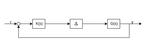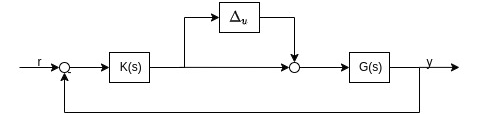
Loop Transfer Function	$L_u = K G \Delta$	$L_u = K G (I_u + \Delta_u)$
Return Difference	$I_u + L_u = I_u + K G \Delta$	$I_u + L_u = I_u + K G (I_u + \Delta_u)$

Gain and Phase Margins For Multivariable Systems at Plant Input

We want to find the smallest uncertainty $\Delta$ that destabilizes the nominal system.

The return difference matrix of Additive Uncertainty Model could be expressed as:

\[\begin{aligned} I_u + KG\Delta &= I_u + L_u\Delta \\ &=[(\Delta^{-1}-I_u)(I_u+L_u)^{-1}+I_u](I_u+L_u)\Delta \end{aligned}\]

Assume controller $K(s)$ stabilizes the nominal plant, and since $\Delta$ is diagonal we have

\[\underbrace{I_u + KG\Delta}_{\text{Singular}} =\underbrace{[(\Delta^{-1}-I_u)(I_u+L_u)^{-1}+I_u]}_{\text{This matrix must be singular}}\underbrace{(I_u+L_u)\Delta}_{\text{Nonsingular}}\]

Using $A+B$ argument:

\[\underbrace{(\Delta^{-1}-I_u)(I_u+L_u)^{-1}}_B+\underbrace{I_u}_A\]

To be nonsingular:

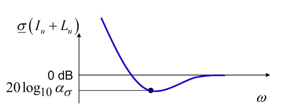
\[\begin{aligned} \underline{\sigma}(A) &> \overline{\sigma}(B)\\ \underline{\sigma}(I_u) &> \overline{\sigma}((\Delta^{-1}-I_u)(I_u+L_u)^{-1})\\ 1 &> \overline{\sigma}((\Delta^{-1}-I_u)(I_u+L_u)^{-1})\\ 1 & \geq \underbrace{\overline{\sigma}(\Delta^{-1}-I_u) \overline{\sigma}((I_u+L_u)^{-1})}_{\text{note that we lose structure here}}\\ \frac{1}{ \overline{\sigma}((I_u+L_u)^{-1})} &\geq \overline{\sigma}(\Delta^{-1}-I_u) \\ \underline{\sigma}(I_u+L_u) &\geq \overline{\sigma}(\Delta^{-1}-I_u) \end{aligned}\]

Let $\alpha_{\sigma} = \displaystyle\min_{w}{ \underline{\sigma}(I_u+L_u(jw))}$,we have

\[\alpha_{\sigma} \geq \overline{\sigma}(\Delta^{-1}-I_u)\\ \sigma_i(\Delta^{-1}-I_u) = |\frac{1}{k_ie^{j\phi_i}}-1|\]

Therefore, stability margin could be computed by:

Gain Margin(zero phase uncertainty $\phi_i = 0^\circ$):

\[\alpha_{\sigma} \geq \overline{\sigma}(\Delta^{-1}-I_u) = |\frac{1}{k_ie^{j\phi_i}}-1|= |\frac{1}{k_i}-1|\\\\ \quad\quad\quad\quad\quad\quad\Downarrow \\\\ \begin{aligned} 1-\alpha_{\sigma} \leq &&\frac{1}{k_i} &&&\leq 1+\alpha_{\sigma}\\ \frac{1}{1+\alpha_{\sigma}} \leq&& k_i &&&\leq \frac{1}{1-\alpha_{\sigma}} \end{aligned}\]

Phase Margin(zero gain uncertainty $k_i = 0$)

\[\begin{aligned} \alpha_{\sigma} \geq \overline{\sigma}(\Delta^{-1}-I_u) & = &&|\frac{1}{k_ie^{j\phi_i}}-1| = |e^{-j\phi_i}-1| = |cos(\phi_i)-1-jsin(\phi_i)|\\ & = &&\sqrt{(cos(\phi_i)-1)^2+sin^2(\phi_i)}\\ & = &&\sqrt{2-2cos(\phi_i))}\\ & = &&\sqrt{4sin^2(\frac{\phi_i}{2})}\\ & = &&\pm2sin(\frac{\phi_i}{2})\\ &\Downarrow \\\\ \phi = \pm2sin^{-1}(\frac{\alpha_{\sigma}}{2}) \end{aligned}\]

Likewise, the return difference matrix of Multiplicative Uncertainty Model could be expressed as:

\[\begin{aligned} I_u + KG(I_u + \Delta_u) &= I_u + L_u(I_u + \Delta_u) = I_u + L_u + L_u\Delta_u \\ &=L_u(L_u^{-1}+I_u+\Delta_u) \end{aligned}\]

Assume controller $K(s)$ stabilizes the nominal plant, we have

\[\underbrace{I_u + KG(I_u + \Delta_u)}_{\text{Singular}} =\underbrace{L_u}_{\text{Nonsingular}}\underbrace{(L_u^{-1}+I_u+\Delta_u)}_{\text{Must be singular}}\]

Using $A+B$ argument:

\[\underbrace{(L_u^{-1}+I_u)}_A + \underbrace{\Delta_u}_B\]

To be nonsingular:

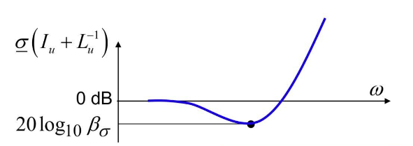
\[\begin{aligned} \underline{\sigma}(A) &> \overline{\sigma}(B)\\ \underline{\sigma}(L_u^{-1}+I_u) &> \overline{\sigma}(\Delta_u)\\ \underline{\sigma}(L_u^{-1}+I_u) &> \overline{\sigma}(\Delta - I_u)\\ \end{aligned}\]

Let $\beta_{\sigma} = \displaystyle\min_{w}{ \underline{\sigma}(I_u+L_u^{-1}(jw))}$, we have

Therefore, stability margin could be computed by:

Gain Margin(zero phase uncertainty $\phi_i = 0^\circ$ ):

\[\beta_{\sigma} \geq \overline{\sigma}(\Delta-I_u) = |k_ie^{j\phi_i}-1|= |k_i-1|\\\\ \quad\quad\quad\quad\quad\quad\Downarrow \\\\ \begin{aligned} 1-\beta{\sigma} \leq &&k_i &&&\leq 1+\beta_{\sigma} \end{aligned}\]

Phase Margin(zero gain uncertainty $k_i = 0$):

\[\begin{aligned} \beta_{\sigma} \geq \overline{\sigma}(\Delta-I_u) & = && |k_ie^{j\phi_i}-1| = |e^{j\phi_i}-1| = |cos(\phi_i)-1+jsin(\phi_i)|\\ & = &&\sqrt{(cos(\phi_i)-1)^2+sin^2(\phi_i)}\\ & = && \sqrt{2-2cos(\phi_i))}\\ & = &&\sqrt{4sin^2(\frac{\phi_i}{2})}\\ & = &&\pm2sin(\frac{\phi_i}{2})\\ &\Downarrow \\\\ \phi = \pm2sin^{-1}(\frac{\beta_{\sigma}}{2}) \end{aligned}\]

Summary of Singular Value Margins:

Also called multivariable stability margins
Both sufficient test for stability
Always more conservative than SISO classical margins

	Additive Uncertainty Model $I+L$	Multiplicative Uncertainty Model $I+L^{-1}$
Gain Margin $GM$	$[\frac{1}{1+\alpha_{\sigma}} \quad \frac{1}{1-\alpha_{\sigma}}]$	$[1-\beta_{\sigma} \quad1+\beta_{\sigma}]$
Phase Margin $PM$	$\pm2sin^{-1}(\frac{\alpha_{\sigma}}{2})$	$\pm2sin^{-1}(\frac{\beta_{\sigma}}{2})$
Best Gain Margin	$[-6 \quad +\infty] \text{ dB}$	$[-\infty \quad +6] \text{ dB}$
Best Phase Margin	$\pm60^\circ$	$\pm60^\circ$
Singular Value Margins	$\begin{aligned}GM_{SV} = GM_{I+L} \cup GM_{I+L^{-1}}\\PM_{SV} = PM_{I+L} \cup PM_{I+L^{-1}}\end{aligned}$	$\begin{aligned}GM_{SV} = GM_{I+L} \cup GM_{I+L^{-1}}\\PM_{SV} = PM_{I+L} \cup PM_{I+L^{-1}}\end{aligned}$

The Control Design Dilemma:

The best gain and phase margin is achieved when $\alpha_{\sigma} = \beta_{\sigma}=1$, as a control engineer, we would like make $\alpha_{\sigma} = \beta_{\sigma}=1$ large at the same time

Return Difference Matrix $I+L=S^{-1}$	Stability Robustness Matrix $I+L^{-1} = T^{-1}$
Inverse of Sensitivity	Inverse of Complementary Sensitivity
$\min_{\omega}\underline{\sigma}(I+L_u)=\alpha_{\sigma} = \frac{1}{\lVert S_u \rVert _{\infty}}$	$\min_{\omega}\underline{\sigma}(I+L_u^{-1})=\beta_{\sigma} = \frac{1}{\lVert T_u \rVert _{\infty}}$

Small minimum singular value indicates poor stability robustness	Small minimum singular value indicates large peak resonance
Make $S$ small at low frequencies for command following	Make $T$ small at high frequencies for robustness to unmodeled dynamics and sensor noise
Equality Constraint	$S+T = I$
Fundamental Trade-off	Must trade-off when neither are small at loop gain crossover frequency

Frequency Domain Analysis

singular value stability robustness analysis

This post is licensed under CC BY 4.0 by the author.

	Additive Uncertainty Model $I+L$	Multiplicative Uncertainty Model $I+L^{-1}$
Gain Margin $GM$	\([\frac{1}{1+\alpha_{\sigma}} \quad \frac{1}{1-\alpha_{\sigma}}]\)	\([1-\beta_{\sigma} \quad1+\beta_{\sigma}]\)
Phase Margin $PM$	\(\pm2sin^{-1}(\frac{\alpha_{\sigma}}{2})\)	\(\pm2sin^{-1}(\frac{\beta_{\sigma}}{2})\)
Best Gain Margin	\([-6 \quad +\infty] \text{ dB}\)	\([-\infty \quad +6] \text{ dB}\)
Best Phase Margin	\(\pm60^\circ\)	\(\pm60^\circ\)
Singular Value Margins	\(\begin{aligned}GM_{SV} = GM_{I+L} \cup GM_{I+L^{-1}}\\PM_{SV} = PM_{I+L} \cup PM_{I+L^{-1}}\end{aligned}\)	\(\begin{aligned}GM_{SV} = GM_{I+L} \cup GM_{I+L^{-1}}\\PM_{SV} = PM_{I+L} \cup PM_{I+L^{-1}}\end{aligned}\)