Frequency Domain Analysis of MIMO System Part 2. Multi-variable Nyquist Theorem
In this post, we show how to analysis robustness of a MIMO system with Multi-variable Nyquist Theorem.
Determinant of Return Difference
The determinant of return difference matrix could be express as
\[\det[RD] = \det\begin{bmatrix}I + L(s)\end{bmatrix} = k \cdot \frac{\phi_{cl}(s)}{\phi_{ol}(s)}\]where $\phi_{ol}(s) ,\phi_{cl}(s)$ is open-loop and closed-loop polynomial respectively.
Proof:
The open-loop poles are given by:
\[\phi_{ol}(s)=\det(sI-A)\]The closed-loop poles are given by:
\[\phi_{cl}(s) = \det(sI-A_{cl})= \det(sI-A+B(I+D)^{-1}C)\]Schur’s determinant lemma states that:
When $A$,respectively $D$ is invertible, then one has
\[\begin{aligned} \det \begin{bmatrix}A&B\\C&D\end{bmatrix}&=\det(A)\cdot\det (D-CA^{-1}B)\\ & = \det(D)\cdot\det(A-BD^{-1}C) \end{aligned}\]define
\[M = \begin{bmatrix}sI-A &B\\-C & I+D\end{bmatrix}\]apply Schur’s determinant lemma, we have:
\[\begin{aligned} \det(M) &= \det(sI-A)\cdot\det(I+D+C(sI-A)^{-1}B) \\ &=\det(sI-A)\cdot\det(I+L) \\ &=\phi_{ol}(s)\cdot\det(I+L)\\ \\ \det(M) &= \det(I+D)\cdot\det(sI-A+B(I+D)^{-1}C) \\ &=\det(I+D)\cdot\phi_{cl}(s) \end{aligned}\]Therefore
\[det(I+L) =det(I+D)\cdot \frac{\phi_{cl}(s)}{\phi_{ol}(s)} = k\cdot \frac{\phi_{cl}(s)}{\phi_{ol}(s)}\]Hence proved
Suppose $D$ is zero matrix, we have
\[det(I+L) = \frac{\phi_{cl}(s)}{\phi_{ol}(s)}\]Multi-variable Nyquist Theorem
Multi-variable Nyquist criterion is derived from Cauchy’s argument principle, it gives a ‘yes or no’ answer to the stability question of closed-loop MIMO system.
It states:
The control system will be closed-loop stable( $\phi_{cl}(s)$ has no RHP zeros) IFF,
$\forall R $ sufficiently large,
\[N(0,\det[I+L(s)],D_R) = -P_{ol}\]or equivalently
\[N(-1,-1+\det[I+L(s)],D_R) = -P_{ol}\]where $N$ is number of encirclements,$D_R$ is Nyquist Contour, $P_{ol}$ is number of open loop unstable poles.
Proof:
Using argument principle, it’s easy to show:
If $f(s)$ is factored where $f(s) = f_1(s)\cdot f_2(s) $ ,then
\[\begin{aligned} N(0,f(s),D_R)&=N(0,f_1(s),D_R)+N(0,f_2(s),D_R)\\ &=(Z_1-P_1) +(Z_2-P_2)=Z-P \end{aligned}\]Suppose a zero $D$ matrix, we have
\[det(I+L) = \frac{\phi_{cl}(s)}{\phi_{ol}(s)}\]Therefore
\[N(0,\phi_{cl}(s),D_R)=N(0,\phi_{ol}(s),D_R)+N(0,\det[I+L],D_R)\]If closed-loop MIMO system is stable, then
\[N(0,\phi_{cl}(s),D_R)=0\]From equation above, the stability of $\phi_{cl}(s)$ requires that
\[N(0,\det[I+L],D_R)=-N(0,\phi_{ol}(s),D_R)=-P_{ol}\]Hence proved
IMPORTANT: Fundamental to this approach is the assumption that the nominal closed-loop system is stable.
Apply to Lateral Control Problem
Since the plant model and controller model is non-square in lateral control problem, so stability analysis should be conducted at the loop break of minimum dimension. In this case, plant input is selected as the loop break point.
How time delay affect closed-loop stability?
A significant deterioration in both gain and phase margin could be observed!
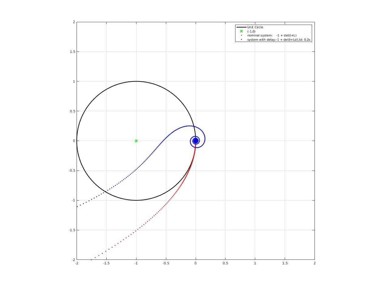 Comparison between stability of nominal closed-loop system and system with delay
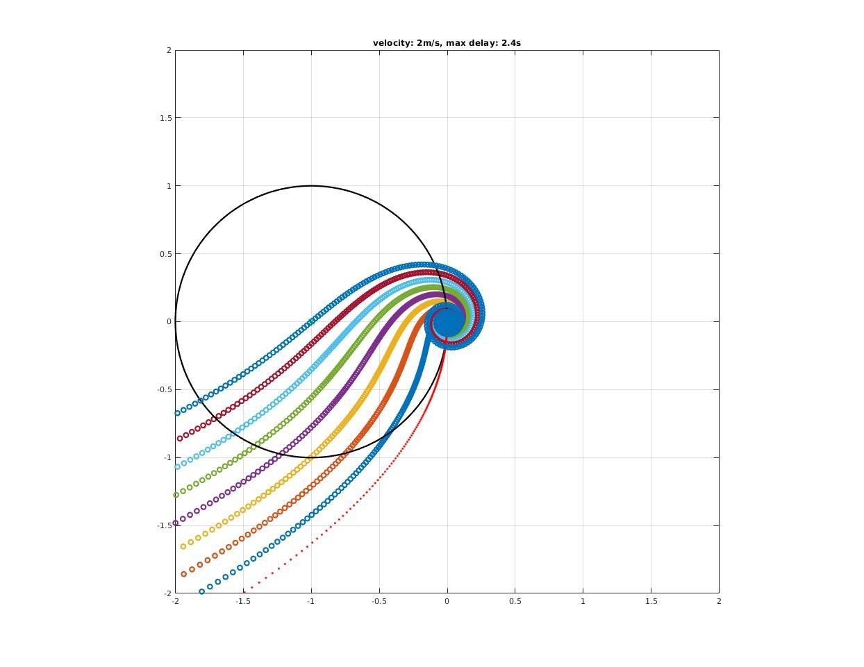
How much pure delay will destabilized the closed-loop system?
Max delay acceptable by closed-loop system could be found where encirclement change as we increase delay time.
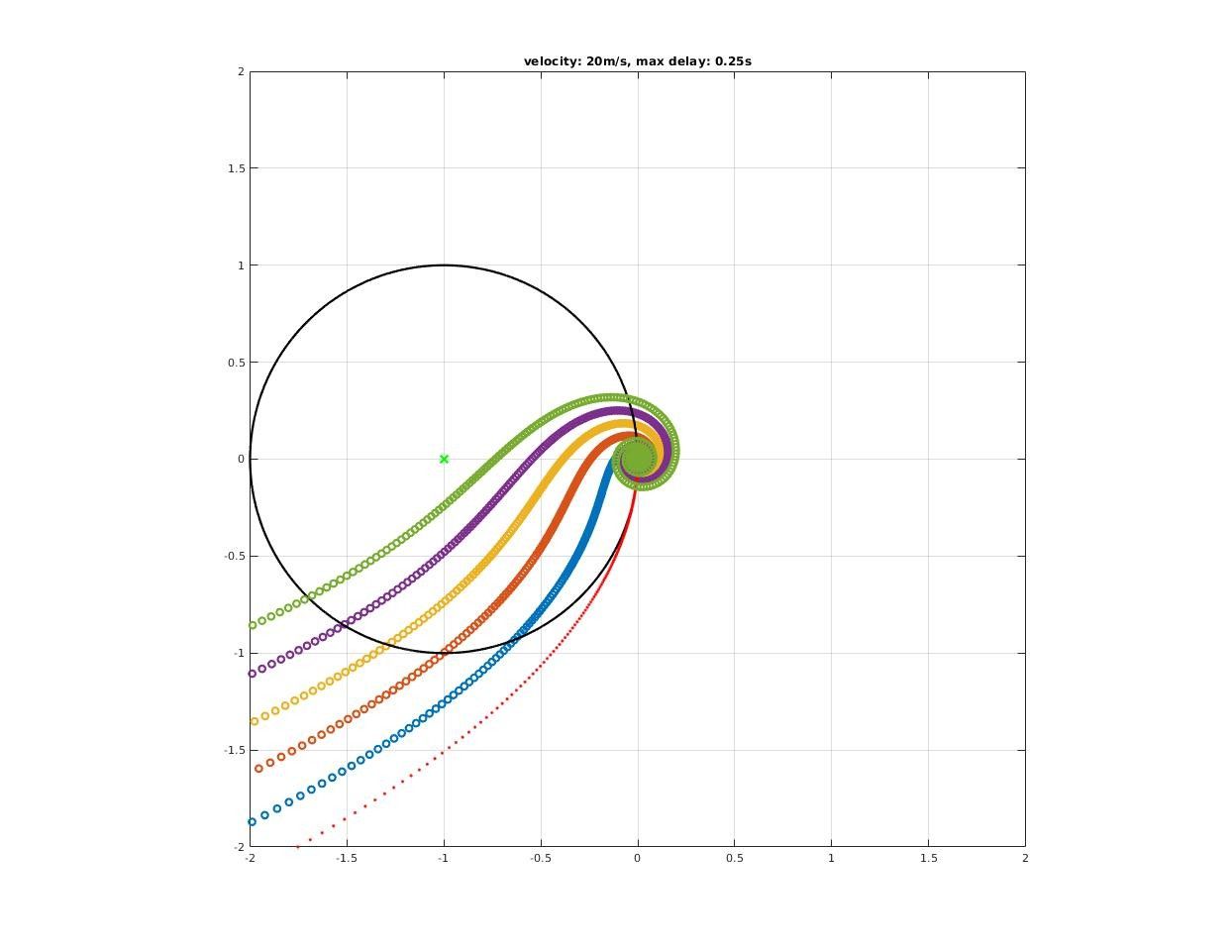
| Model Velocity (m/s) | Nyquist Plot | Max Delay (s) |
|---|---|---|
| 1 | 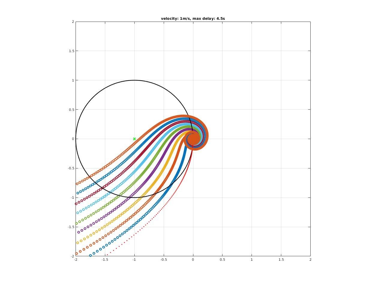 | 4.5 |
| 2 | | 2.4 |
| 4 | 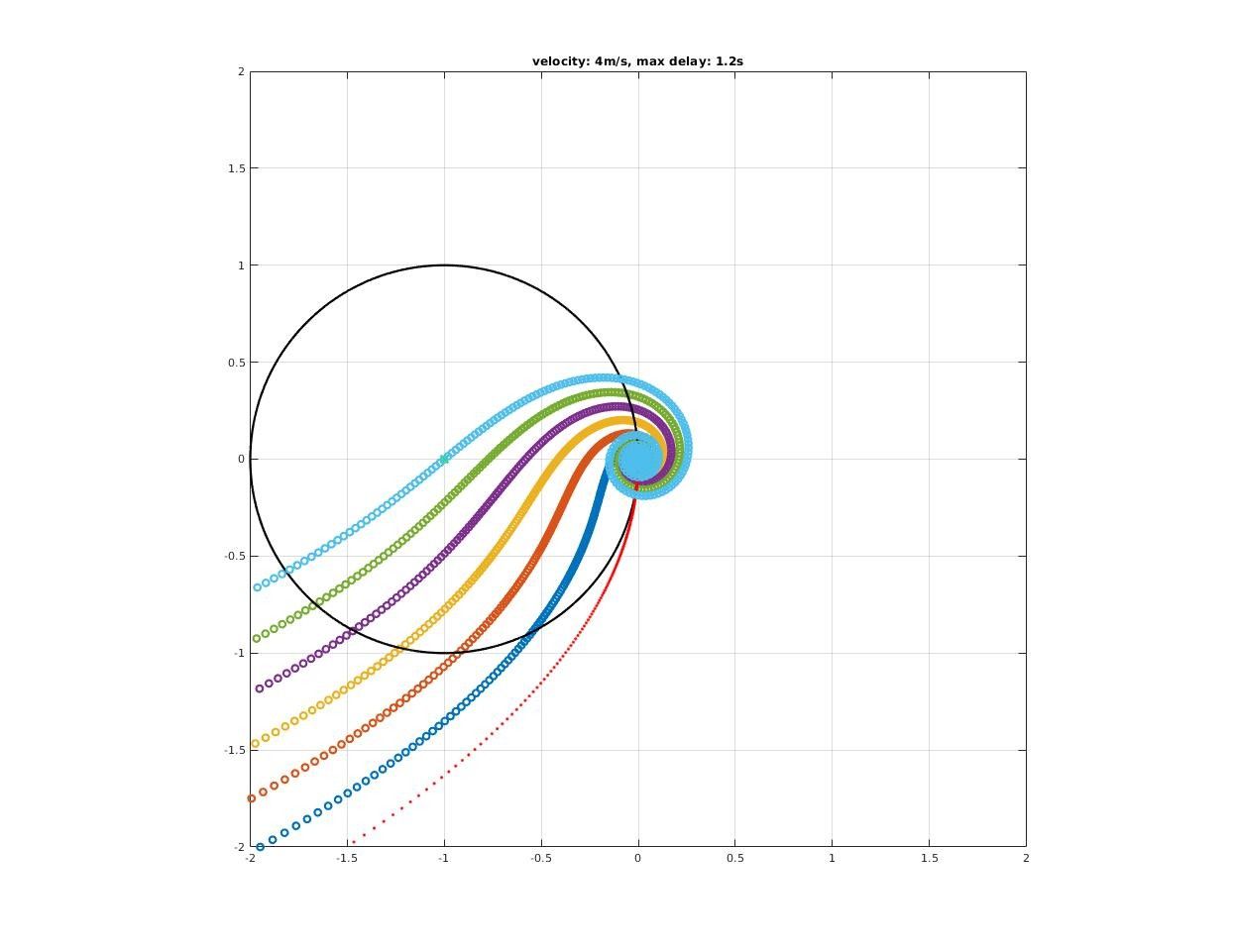 | 1.2 |
| 8 | 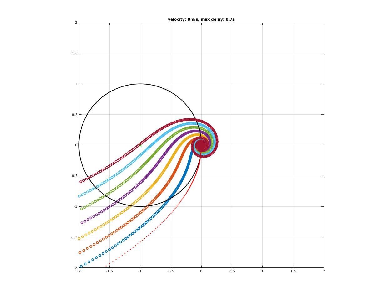 | 0.7 |
| 12 | 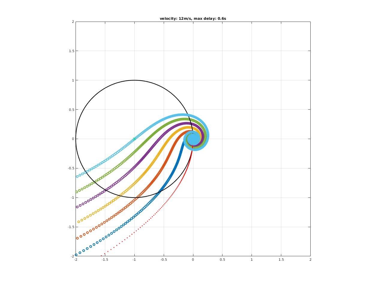 | 0.6 |
| 16 | 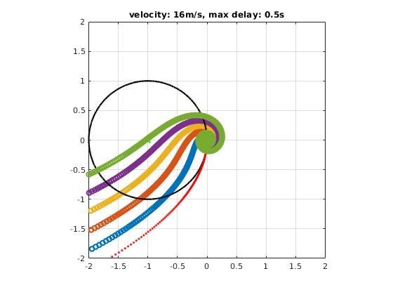 | 0.5 |
| 20 | 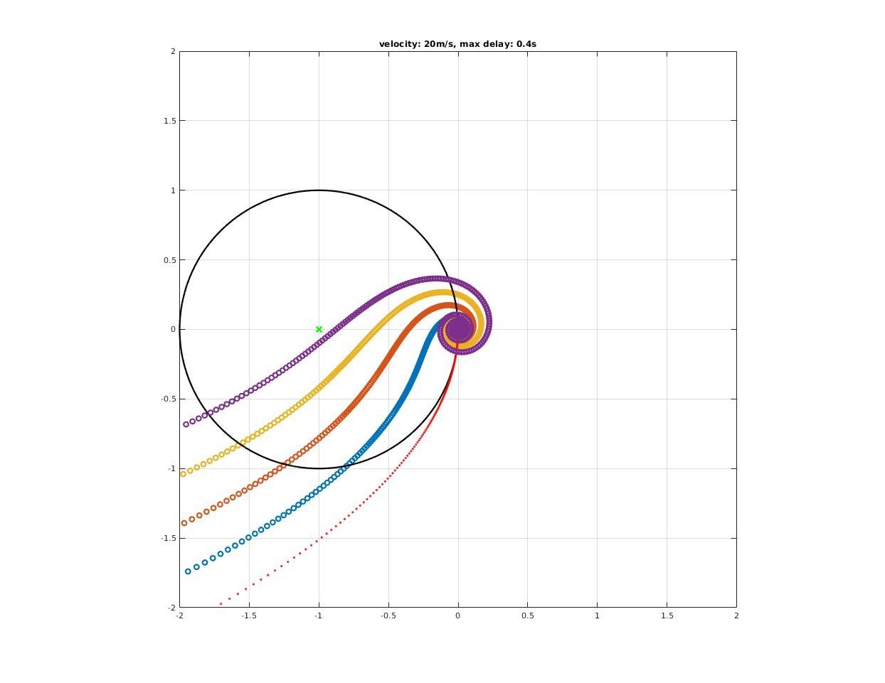 | 0.4 |
| 25 |  | 0.4 |
| 30 | 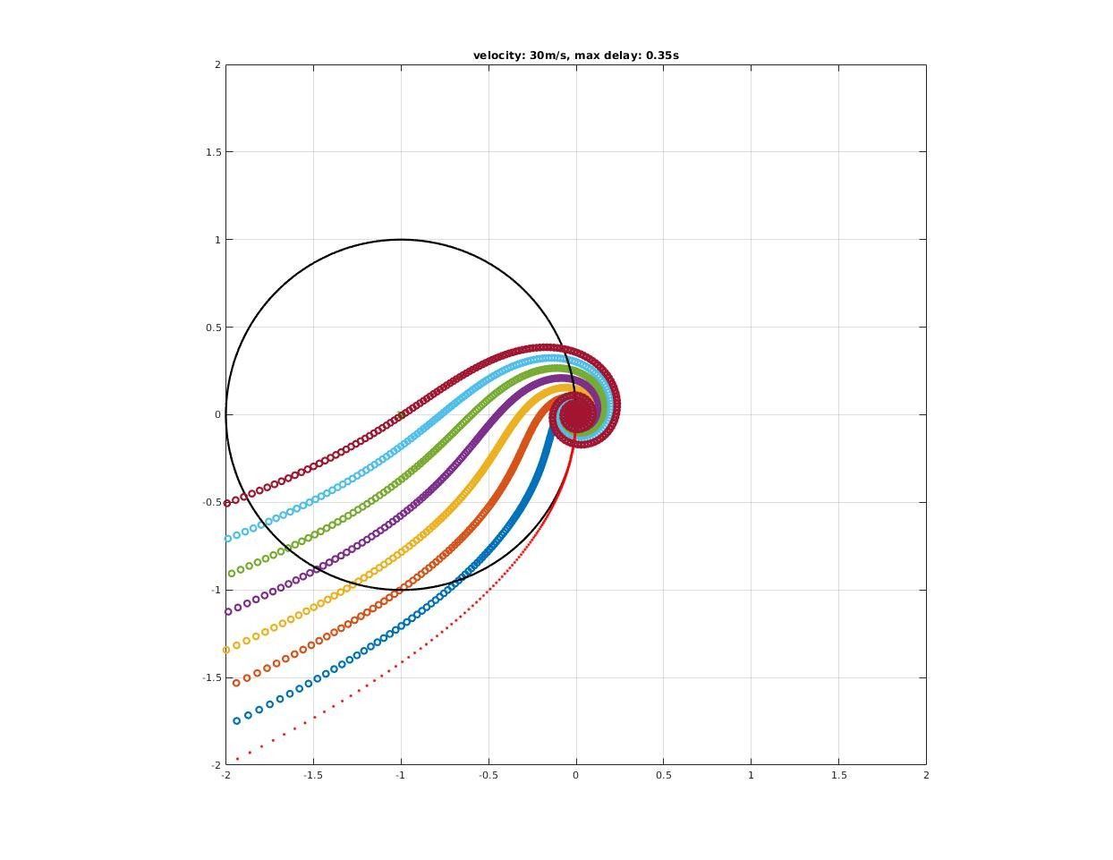 | 0.35 |
How actuator dynamics affect closed-loop system?
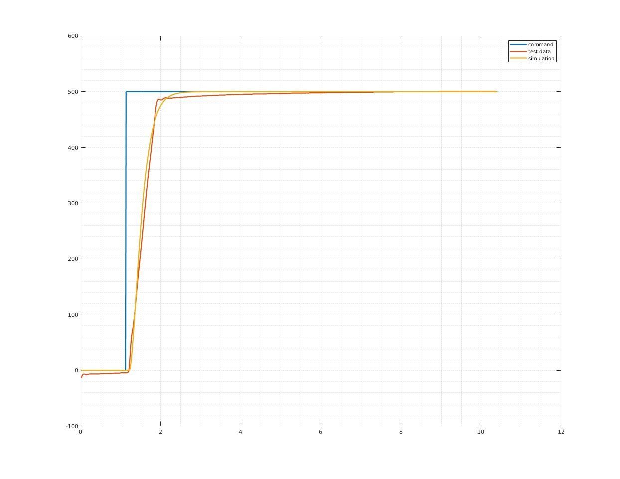
First, construct a actuator model from road test data
The actuator model I used in analysis is a pure delay + second order system:
\[f(s) = e^{-t_ds}\cdot\frac{w_n^2}{s^2+2\eta w_n s + w_n^2}\]where
\[\begin{cases} t_d &= 0.1\;s\\ w_n &= 6.0 \;rad/s\\ \eta &= 1.0\\ \end{cases}\]Step response comparison between real system and simulation system:
Then, we add actuator dynamics into plant model, reconnect it with controller and analysis frequency response of closed-loop system. Here’s what we get:
| Model Velocity (m/s) | Nyquist Plot | Gain Crossover Frequency (Hz) | Gain Margin (dB) | Phase Margin (deg) | Extra Max Delay (s) |
|---|---|---|---|---|---|
| 1 | 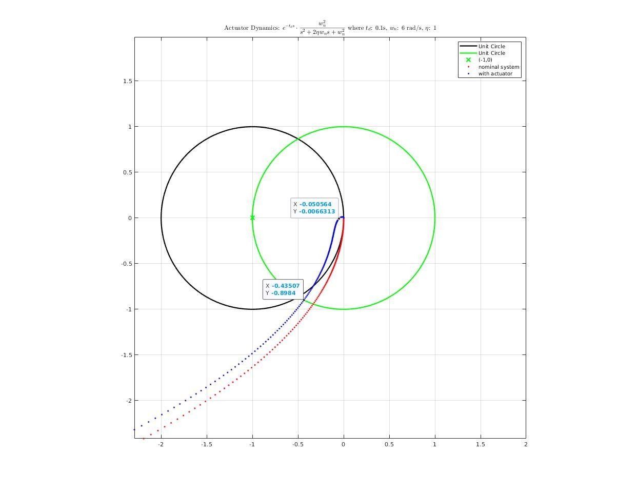 | 0.05 | 25.9 | 64.2 | 4.3 |
| 5 | 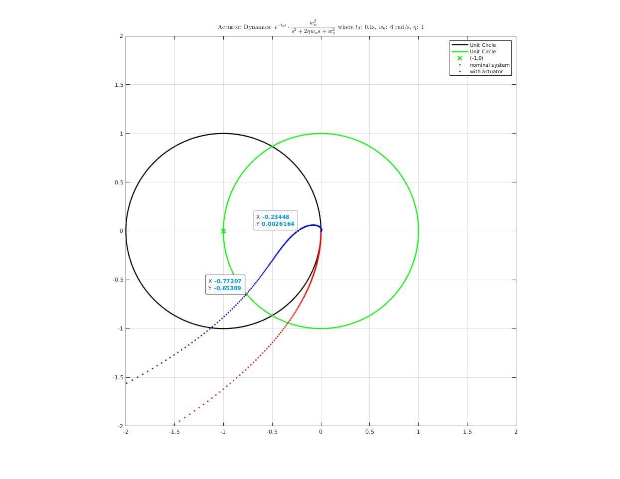 | 0.19 | 12.6 | 40.3 | 0.6 |
| 10 | 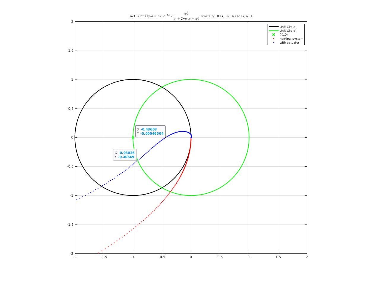 | 0.29 | 7.21 | 23.6 | 0.2 |
| 15 | 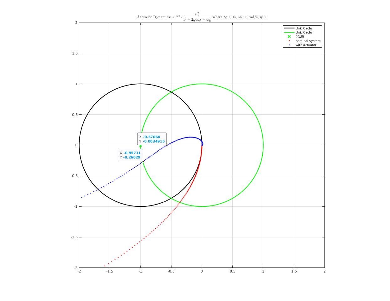 | 0.34 | 4.87 | 15.5 | 0.14 |
| 20 | 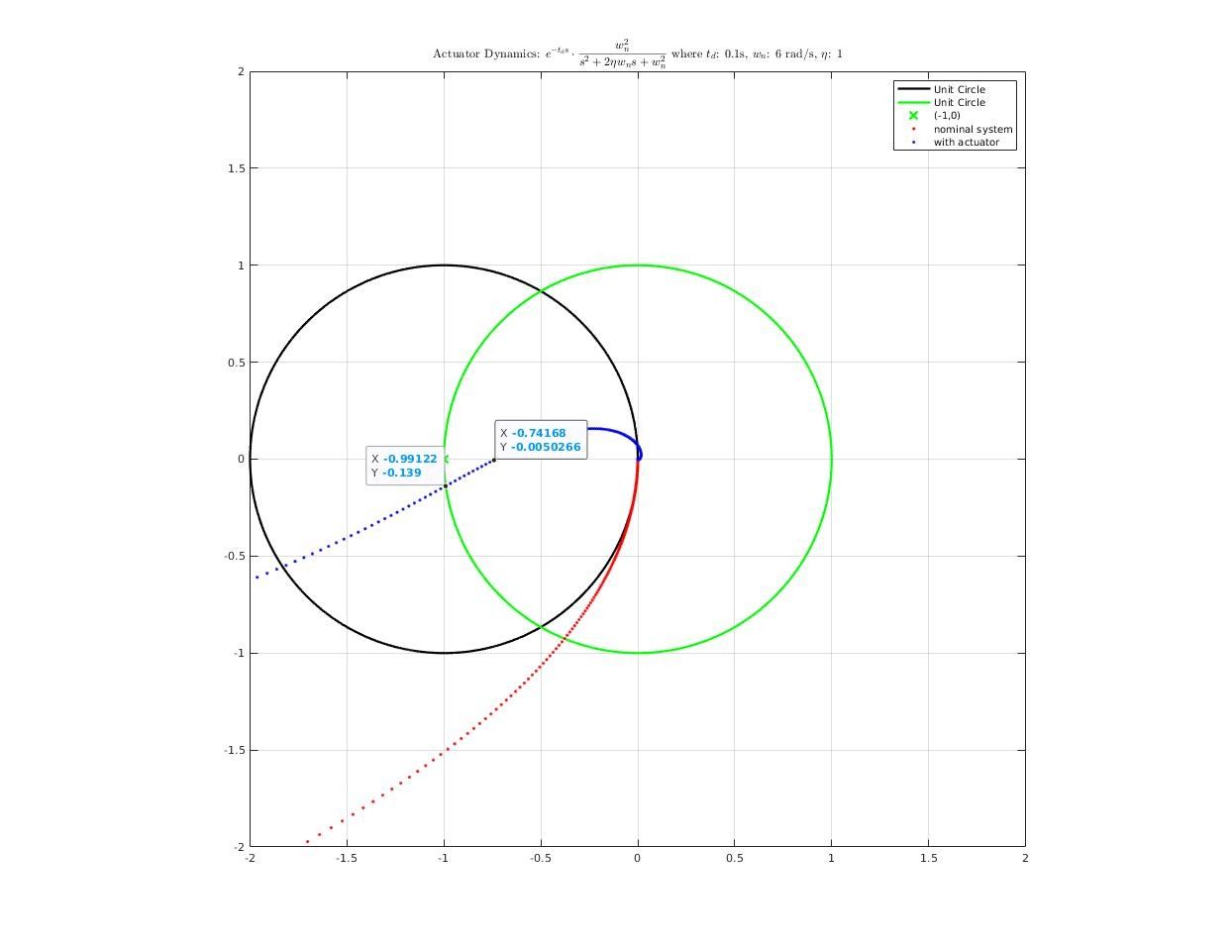 | 0.38 | 2.60 | 7.98 | 0.06 |
| 25 | 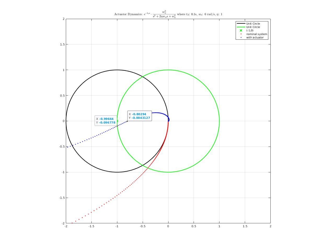 | 0.39 | 1.91 | 5.55 | 0.04 |
| 30 | 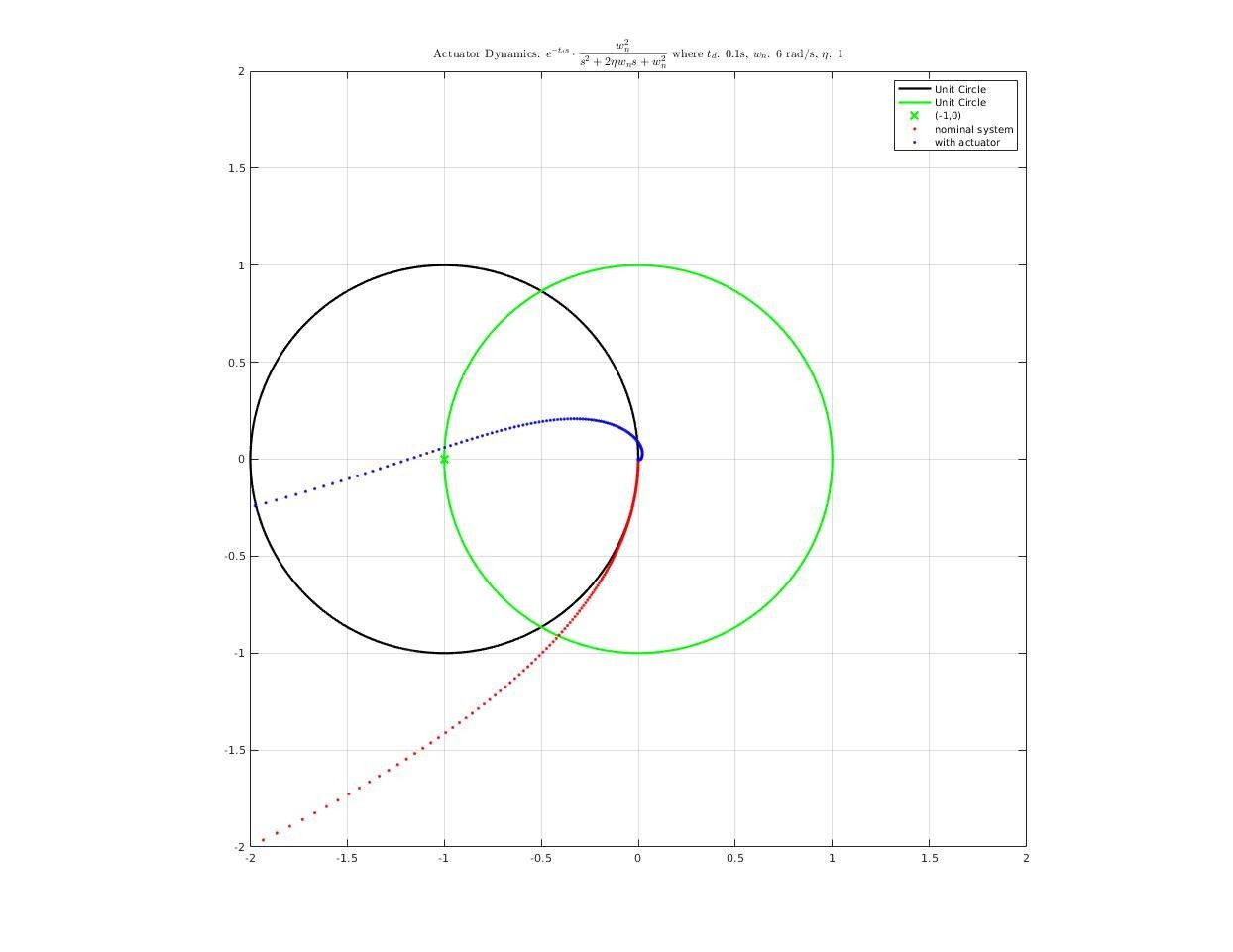 | unstable | unstable | unstable | unstable |
Summary
The Multi-variable Nyquist Criterion gives a ‘yes or no’ answer to the stability question of a MIMO system. Understanding it leads to important understanding of the robustness analysis tests used to analyze model uncertainties. In addition, stability margins for MIMO systems can be derived using the MNT by assuming that controller $K(s)$ stabilizes the nominal plant $G(s)$ and that gain and phase uncertainties are large enough to change the number of encirclements made by the determinant of the return difference matrix locus.