Frequency Domain Analysis of MIMO System Part 1. Model Generalization

In this post, we present a generalized state-space linear-time-invariant plant and controller models for control design and frequency domain analysis that will be used in other sections. Models for closed-loop simulation and frequency domain analysis at both plant input and plant output are also derived.

System Modeling

Our goal is to convert system dynamics and controllers into a common framework for analysis and comparison.

The plant model is:

\[\begin{aligned} \dot{x} &= A_p x + B_p u \\ y &= C_p x +D_p u \end{aligned}\]

where

\[x \in R ^{n_x \cdot 1}, u \in R ^{n_u \cdot 1}, y \in R^{n_y \cdot 1}\]

and

\[\begin{aligned} A_p \in R^{n_x \cdot n_x} , B_p\in R^{n_x \cdot n_u} \\ C_p \in R^{n_y \cdot n_x} ,D_p\in R^{n_y \cdot n_u} \\ \end{aligned}\]

The controller model is:

\[\begin{aligned} \dot{x}_c &= A_c x_c + B_{c_1} y + B_{c_2}r\\ u &= C_c x_c + D_{c_1} y + D_{c_2}r \end{aligned}\]

where

\[x_c \in R^{n_{x_c} \cdot 1}, \quad u \in R^{n_u \cdot 1}, \quad y \in R^{n_y \cdot 1},\quad r \in R^{n_r \cdot 1} \\ \\\]

and

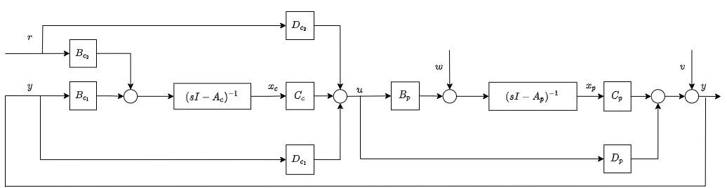
\[\begin{aligned} &A_c \in R^{n_{x_c}\cdot n_{x_c}}, \quad &&B_{c_1}\in R^{n_{x_c} \cdot n_y},\quad &&& B_{c_2}\in R^{n_{x_c} \cdot n_r} \\ &C_c \in R ^{n_u \cdot n_{x_c}}, \quad &&D_{c_1}\in R^{n_u \cdot n_y},\quad &&& D_{c_2}\in R^{n_u \cdot n_r} \end{aligned}\]

The plant and controller is connected as shown in following block diagram:

Derivation of Closed-loop Dynamics

rewrite $u$ by replacing plant output $y$, we have

\[\begin{aligned} &&u&=C_c x_c + D_{c_1}y+ D_{c_2}r\\ && &= C_c x_c + D_{c_1}(C_p x + D_p u) + D_{c_2}r\\ && &= C_c x_c +D_{c_1}C_px +D_{c_1}D_pu + D_{c_2}r\\ \\ && \underbrace{(I-D_{c_1}D_p)}_{Z} u &= C_c x_c +D_{c_1}C_px + D_{c_2}r \\ && u &= Z^{-1}(C_c x_c +D_{c_1}C_px + D_{c_2}r) \end{aligned}\]

feed $u$ into the plant, we have:

\[\begin{aligned} \dot{x} &= A_p x + B_p Z^{-1}(C_cx_c + D_{c_1}C_px + D_{c_2}r) \\ &=A_px + B_pZ^{-1}C_cx_c + B_pZ^{-1}D_{c_1}C_px + B_pZ^{-1}D_{c_2}r \\ &=(A_p + B_pZ^{-1}D_{c_1}C_p)x + B_pZ^{-1}C_cx_c + B_pZ^{-1}D_{c_2}r \end{aligned}\]

likewise:

\[\begin{aligned} \dot{x}_c &= A_cx_c + B_{c_1}(C_px+D_pu) +B_{c_2}r\\ &=A_cx_c + B_{c_1}C_px +B_{c_1}D_pZ^{-1}(C_cx_c+D_{c_1}C_px+D_{c_2}r)+B_{c_2}r\\ &=(A_c+B_{c_1}D_pZ^{-1}C_c)x_c + (B_{c_1}C_p+B_{c_1}D_pZ^{-1}D_{c_1}C_p)x+(B_{c_1}D_pZ^{-1}D_{c_2}+B_{c_2})r\\ &=(A_c+B_{c_1}D_pZ^{-1}C_c)x_c + B_{c_1}(I+D_pZ^{-1}D_{c_1})C_px+(B_{c_1}D_pZ^{-1}D_{c_2}+B_{c_2})r\\ \\ y &= C_px+D_pu \\ &= C_px + D_p Z^{-1}(C_cx_c+D_{c_1}C_px +D_{c_2}r)+B_{c_2}r\\ &= (C_p + D_p Z^{-1}D_{c_1}C_p)x + D_p Z^{-1}C_cx_c + D_p Z^{-1}B_{c_2}r\\ &=(I+D_pZ^{-1}D_{c_1})C_px + D_p Z^{-1}C_cx_c + D_p Z^{-1}B_{c_2}r \end{aligned}\]

Let us define a augmented state vector $x_a$ in the form:

\[\begin{aligned} x_a = \begin{bmatrix} x\\x_c \end{bmatrix} \end{aligned}\]

Then, the closed-loop dynamics can be written as:

\[\begin{aligned} \begin{bmatrix}\dot{x}\\\dot{x}_c\end{bmatrix} &=&&\underbrace{ \begin{bmatrix}A_p+B_pZ^{-1}D_{c_1}C_p & B_pZ^{-1}C_c \\ B_{c_1}(I+D_pZ^{-1}D_{c_1})C_p & A_c+B_{c_1}D_pZ^{-1}C_c\end{bmatrix}}_{A_{cl}}\begin{bmatrix}x\\x_c\end{bmatrix} + \underbrace{ \begin{bmatrix}B_pZ^{-1}D_{c_2}\\B_{c_1}D_pZ^{-1}D_{c_2}+B_{c_2}\end{bmatrix}}_{B_{cl}}r\\\\ y &=&& \underbrace{ \begin{bmatrix}(I+D_pZ^{-1}D_{c_1})C_p & D_pZ^{-1}C_c\end{bmatrix}}_{C_{cl}}\begin{bmatrix}x\\ x_c\end{bmatrix}+\underbrace{ \begin{bmatrix}D_pZ^{-1}D_{c_2}\end{bmatrix}}_{D_{cl}}r \end{aligned}\]

or equivalently

\[\begin{aligned} \dot{x}_a &= A_{cl} x_a + B_{cl}r \\ y&= C_{cl}x_a+D_{cl}r \end{aligned}\]

Loop Gain at Plant Input and Plant Output

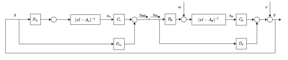
The loop gain model at the plant input is formed to support frequency domain analysis of the design at the plant input loop break point. In this model, we treat the control input to the plant as the model input $u_{in}$ .The control output from the controller becomes the model output $u_{out}$ .Also,we neglect the command vector $r$. In this case, the plant and controller models are:

\[\begin{aligned} \dot{x} &=&& A_p x + B_p u_{in} , \quad &&&\dot{x}_c &&&&= A_c x_c +B_{c_1}y\\ y &=&& C_p x + D_p u_{in} , \quad &&&u_{out} &&&&= C_cx_c + D_{c_1}y \end{aligned}\]

Then we connect these two system with as input $u_{in}$ and as output $u_{out}$ as shown below

We can show that

\[\begin{aligned} \dot{x}_c &=&& A_c x_c + B_{c_1}y \\ &=&&A_cx_c + B_{c_1}(C_px + D_pu_{in})\\ &=&&A_cx_c + B_{c_1}C_px + B_{c_1}D_pu_{in}\\\\ u_{out} &= &&C_cx_c +D_{c_1}y \\ &=&&C_cx_c +D_{c_1}(C_px + D_pu_{in})\\ &=&&C_cx_c +D_{c_1}C_px + D_{c_1}D_pu_{in} \end{aligned}\]

Rewrite these relations in matrix form:

\[\begin{aligned} \begin{bmatrix}\dot{x}\\\dot{x}_c\end{bmatrix} &=&&\underbrace{ \begin{bmatrix}A_p &0 \\B_{c_1}C_p & A_c\end{bmatrix}}_{A_{lu}}\begin{bmatrix}x\\x_c\end{bmatrix} + \underbrace{ \begin{bmatrix}B_p \\B_{c_1}D_p\end{bmatrix}}_{B_{lu}}u_{in}\\\\ u_{out} &=&& \underbrace{ \begin{bmatrix}D_{c_1}C_p &C_c\end{bmatrix}}_{C_{lu}}\begin{bmatrix}x\\ x_c\end{bmatrix}+\underbrace{ \begin{bmatrix}D_{c_1}D_p\end{bmatrix}}_{D_{lu}}u_{in} \end{aligned}\]

The loop gain matrix at the plant input is

\[L_{u}(s) = C_{lu}(sI-A_{lu})^{-1}B_{lu}+D_{lu}\]

The return difference matrix at the plant input is

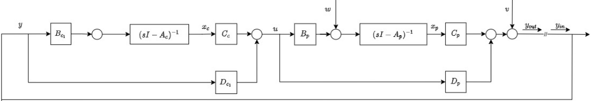
\[RD_{u} = \frac{u_{in} - u_{out}}{u_{in}}= \frac{u_{in} - (-L_{u}u_{in})}{u_{in}} = I+L_{u}\]

Similarly, the loop gain model at the plant output is formed to support frequency domain analysis of the design at the plant output loop break point. In this model, we treat the plant output feeding to the controller as the model input $y_{in}$.The plant output from the plant becomes the model output $y_{out}$ .And neglect the command vector $r$ . In this case, the plant and controller models are:

\[\begin{aligned} \dot{x} &=&& A_p x + B_p u , \quad &&&\dot{x}_c &&&&= A_c x_c +B_{c_1}y_{in}\\ y_{out} &=&& C_p x + D_p u , \quad &&&u &&&&= C_cx_c + D_{c_1}y_{in} \end{aligned}\]

Then we connect these two system with $y_{in}$ as input and $y_{out}$ as output as shown below

We can show that

\[\begin{aligned} \dot{x} &=&& A_p x + B_pu \\ &=&& A_p x + B_p(C_cx_c + D_{c_1}y_{in})\\ &=&& A_p x + B_pC_cx_c + B_pD_{c_1}y_{in}\\\\ y_{out} &= &&C_px +D_pu \\ &=&&C_px +D_p(C_cx_c + D_{c_1}y_{in})\\ &=&&C_px +D_pC_cx_c + D_pD_{c_1}y_{in} \end{aligned}\]

Rewite these relations in matrix form:

\[\begin{aligned} \begin{bmatrix}\dot{x}\\\dot{x}_c\end{bmatrix} &=&\underbrace{ \begin{bmatrix}A_p &B_pC_c \\0 & A_c\end{bmatrix}}_{A_{ly}}\begin{bmatrix}x\\x_c\end{bmatrix} + \underbrace{ \begin{bmatrix}B_pD_{c_1} \\B_{c_1}\end{bmatrix}}_{B_{ly}}y_{in}\\\\ y_{out} &=& \underbrace{ \begin{bmatrix}C_p &D_pC_c\end{bmatrix}}_{C_{ly}}\begin{bmatrix}x\\ x_c\end{bmatrix}+\underbrace{ \begin{bmatrix}D_pD_{c_1}\end{bmatrix}}_{D_{ly}}y_{in} \end{aligned}\]

The loop gain matrix at the plant output is

\[L_{y}(s) = C_{ly}(sI-A_{ly})^{-1}B_{ly}+D_{ly}\]

The return difference matrix at the plant output is

\[RD_{y} = \frac{y_{in} - y_{out}}{y_{in}}= \frac{y_{in} - (-L_{y}y_{in})}{y_{in}} = I+L_{y}\]

Summary

Closed-loop Dynamics

State space model:

\[\begin{aligned} \dot{x}_a &= A_{cl} x_a + B_{cl}r \\ y&= C_{cl}x_a+D_{cl}r \end{aligned}\]

where

\[\begin{aligned} A_{cl}&=&&\begin{bmatrix}A_p+B_pZ^{-1}D_{c_1}C_p & B_pZ^{-1}C_c \\ B_{c_1}(I+D_pZ^{-1}D_{c_1})C_p & A_c+B_{c_1}D_pZ^{-1}C_c\end{bmatrix}\\ B_{cl}&=&& \begin{bmatrix}B_pZ^{-1}D_{c_2}\\B_{c_1}D_pZ^{-1}D_{c_2}+B_{c_2}\end{bmatrix}\\ C_{cl} &=&& \begin{bmatrix}(I+D_pZ^{-1}D_{c_1})C_p & D_pZ^{-1}C_c\end{bmatrix}\\ D_{cl} &=&&\begin{bmatrix}D_pZ^{-1}D_{c_2}\end{bmatrix} \end{aligned}\]

Characteristic at Plant Input and Plant Output

	Plant Input	Plant Output
State Space Model	\(\begin{aligned}\dot{x}_a &= A_{lu} x_a + B_{lu}u_{in} \\ u_{out}&= C_{lu}x_a+D_{lu}u_{in}\end{aligned}\)	\(\begin{aligned}\dot{x}_a &= A_{ly} x_a + B_{ly}y_{in} \\y_{out}&= C_{ly}x_a+D_{ly}y_{in}\end{aligned}\)
State Space Matrix	\(\begin{aligned}A_{lu} &=&& \begin{bmatrix}A_p &0 \\B_{c_1}C_p & A_c\end{bmatrix}\\B_{lu} &=&& \begin{bmatrix}B_p \\B_{c_1}D_p\end{bmatrix}\\C_{lu} &=&& \begin{bmatrix}D_{c_1}C_p &C_c\end{bmatrix} \\D_{lu} &=&& \begin{bmatrix}D_{c_1}D_p\end{bmatrix}\end{aligned}\)	\(\begin{aligned} A_{ly}&=&&\begin{bmatrix}A_p &B_pC_c \\0 & A_c\end{bmatrix} \\B_{ly}&=&& \begin{bmatrix}B_pD_{c_1} \\B_{c_1}\end{bmatrix}\\ C_{ly}&=&& \begin{bmatrix}C_p &D_pC_c\end{bmatrix}\\D_{ly}&=&&\begin{bmatrix}D_pD_{c_1}\end{bmatrix}\end{aligned}\)
Loop Gain $L(s)$	\(K(s)G(s) = \\ \quad C_{lu}(sI-A_{lu})^{-1}B_{lu}+D_{lu}\)	\(G(s)K(s) = \\ \quad C_{ly}(sI-A_{ly})^{-1}B_{ly}+D_{ly}\)
Return Difference $RD(s)$	\(I+L_u\)	\(I+L_y\)
Sensitivity $S(s)$	\((I+L_u)^{-1}\)	\((I+L_y)^{-1}\)
Complementary Sensitivity $T(s)$	\((I+L_u)^{-1}L_u\)	\((I+L_y)^{-1}L_y\)